Prurigo Nodularis
Background
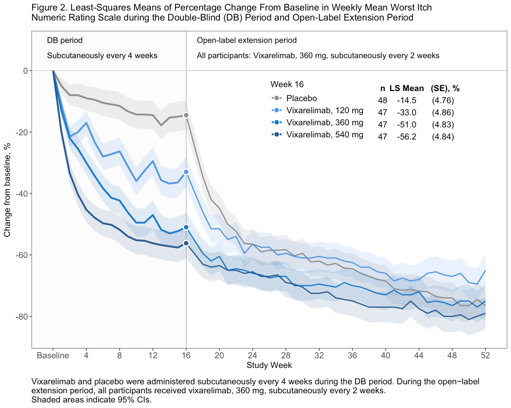
In the recent publication “Vixarelimab in Patients With Prurigo Nodularis: A Randomized Clinical Trial” (DOI: 10.1001/jamadermatol.2025.4950) the study results were presented using the following plot:
Figure 2. Least-Squares Means of Percentage Change From Baseline in Weekly Mean Worst Itch Numeric Rating Scale during the Double-Blind (DB) Period and Open-Label Extension Period
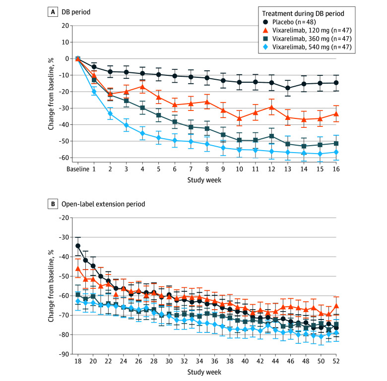
Footnote: Patients who received placebo in the DB period received vixarelimab, 360 mg, subcutaneously once every 2 weeks during the open-label extension period. Error bars indicate 95% CIs.
Importance: Prurigo nodularis (PN) is a chronic inflammatory skin disease characterized by severe pruritus and nodule formation, significantly affecting patients’ quality of life. There is an unmet need for effective therapies to address both symptoms and disease progression.
Challenge
Observe the plot and evaluate the design decisions made. Check what graphical principles can be used to improve the plot. Ask yourself: What is the main message? And how can this be visually supported?
Visualisations
One submission was received for this challenge. During the webinar, step-by-step improvements moving from the original visualisation to the final submission were presented and discussed. Each step is presented below, along with notes on what is changed each time.
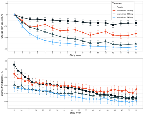
Rebuild of the original visualisation
- The original visualisation is recreated using simulated data
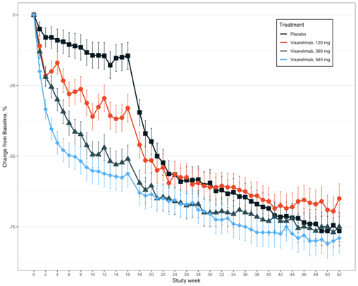
Simplify by combining plots
- Reduce cognitive load
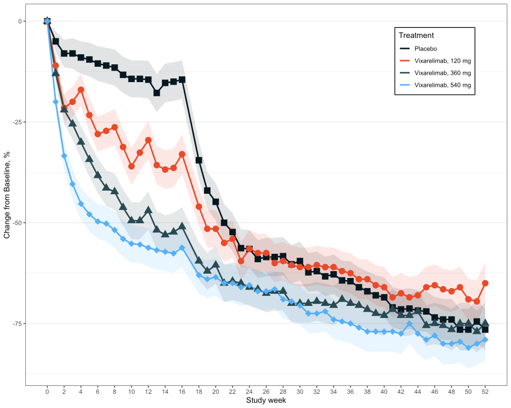
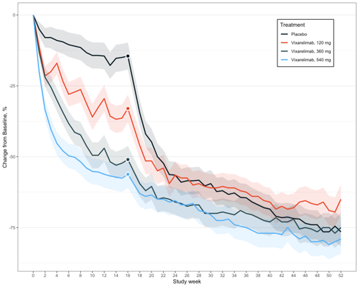
Eliminate clutter - add clarity
- Shaded bands instead of error bars
Eliminate clutter - focus attention
- Remove markers except for Week 16
- White outline
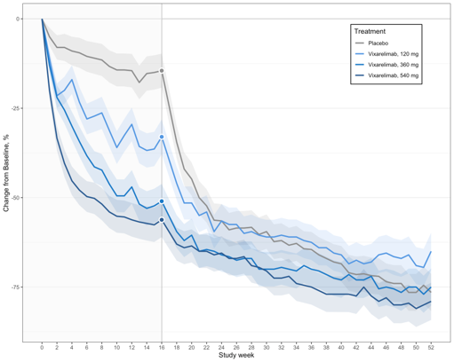
Colour shading
- Reduce cognitive load
- Placebo in grey
- Doses in shades of blue
- Grey line at Week 16
- Area shading
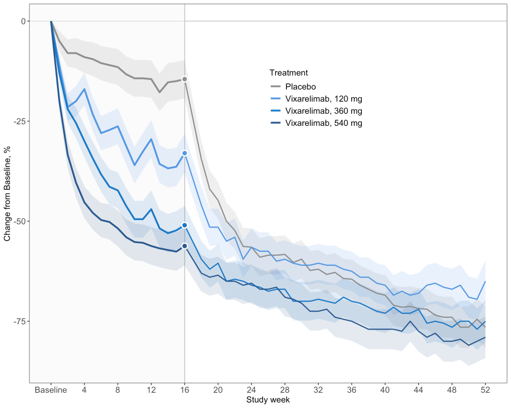
Eliminate clutter - clarity and focus
- Open-label lines thinner and slightly greyed
- Fewer x-axis tick marks
- Grid lines removed
Information
- Title, footnotes and area labels
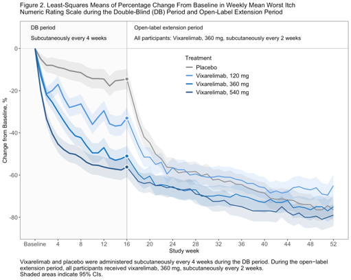
Additional details (Final submission)
- Table with additional information
Code
# libraries
library(ggplot2)
library(cowplot)
library(gridExtra)
library(dplyr)
#import
# study_data <- read.excel("simulated_study_data.xlsx)

#### rebuild original plot (1) ####

p1_a <- ggplot(
  study_data |> dplyr::filter(Week <= 16),
  aes(
    x = Week,
    y = Mean,
    colour = Arm,
    group = Arm
  )
) +
  geom_errorbar(
    aes(
      ymin = Low,
      ymax = High
    ),
    width = 0.25,
    linewidth = 0.4
  ) +
  geom_line(linewidth = 1) +
  geom_point(aes(shape = Arm), size = 4, show.legend = FALSE) +
  scale_colour_manual(
    values = c(
      "Placebo" = "#081820",
      "Vixarelimab, 120 mg"   = "#EA4928",
      "Vixarelimab, 360 mg"   = "#284A52",
      "Vixarelimab, 540 mg"   = "#54B1F9"
    )
  ) +
  scale_x_continuous(
    breaks = seq(0, 16, 1)
  ) +
  labs(
    x = "Study week",
    y = "Change from Baseline, %",
    colour = "Treatment"
  ) +
  theme_bw() +
  theme(
    legend.position = "bottom"
  ) +
  theme(
    legend.position = c(0.85, 0.81),
    legend.background = element_rect(
      fill = "white",
      colour = "black"
    ),
    legend.box.background = element_rect(
      colour = "black"
    ),

    # X-Gridlines entfernen
    panel.grid.major.x = element_blank(),
    panel.grid.minor.x = element_blank()
  ) +
  coord_cartesian(
    ylim = c(-60, 20)
  ) +
  scale_shape_manual(
    values = c(
      "Placebo" = 15,  # Quadrat
      "Vixarelimab, 120 mg"   = 16,  # Kreis
      "Vixarelimab, 360 mg"   = 17,  # Dreieck
      "Vixarelimab, 540 mg"   = 18   # Diamant
    )
  )

p1_a

p1_b <- ggplot(
  study_data |> dplyr::filter(Week >= 18),
  aes(
    x = Week,
    y = Mean,
    colour = Arm,
    group = Arm
  )
) +
  geom_errorbar(
    aes(
      ymin = Low,
      ymax = High
    ),
    width = 0.25,
    linewidth = 0.4
  ) +
  geom_line(linewidth = 1, show.legend = FALSE) +
  geom_point(aes(shape = Arm), size = 4, show.legend = FALSE) +
  scale_colour_manual(
    values = c(
      "Placebo" = "#081820",
      "Vixarelimab, 120 mg"   = "#EA4928",
      "Vixarelimab, 360 mg"   = "#284A52",
      "Vixarelimab, 540 mg"   = "#54B1F9"
    )
  ) +
  scale_x_continuous(
    breaks = seq(18, 52, 2)
  ) +
  labs(
    x = "Study week",
    y = "Change from Baseline, %",
    colour = "Treatment"
  ) +
  theme_bw() +
  theme(
    legend.position = "none"
  ) +
  theme(
    # X-Gridlines entfernen
    panel.grid.major.x = element_blank(),
    panel.grid.minor.x = element_blank()
  ) +
  scale_shape_manual(
    values = c(
      "Placebo" = 15,  # Quadrat
      "Vixarelimab, 120 mg"   = 16,  # Kreis
      "Vixarelimab, 360 mg"   = 17,  # Dreieck
      "Vixarelimab, 540 mg"   = 18   # Diamant
    )
  )
p1_b

p1 <- plot_grid(
  p1_a,
  p1_b,
  ncol = 1,
  align = "v"
)

p1
#### merge to one plot (2) ####

p2 <- ggplot(
  study_data,
  aes(
    x = Week,
    y = Mean,
    colour = Arm,
    group = Arm
  )
) +
  geom_errorbar(
    aes(
      ymin = Low,
      ymax = High
    ),
    width = 0.25,
    linewidth = 0.4
  ) +
  geom_line(linewidth = 1) +
  geom_point(aes(shape = Arm), size = 4, show.legend = FALSE) +
  scale_colour_manual(
    values = c(
      "Placebo" = "#081820",
      "Vixarelimab, 120 mg"   = "#EA4928",
      "Vixarelimab, 360 mg"   = "#284A52",
      "Vixarelimab, 540 mg"   = "#54B1F9"
    )
  ) +
  scale_x_continuous(
    breaks = seq(0, 52, 2)
  ) +
  labs(
    x = "Study week",
    y = "Change from Baseline, %",
    colour = "Treatment"
  ) +
  theme_bw() +
  theme(
    legend.position = "bottom"
  ) +
  theme(
    legend.position = c(0.85, 0.85),
    legend.background = element_rect(
      fill = "white",
      colour = "black"
    ),
    legend.box.background = element_rect(
      colour = "black"
    ),

    # X-Gridlines entfernen
    panel.grid.major.x = element_blank(),
    panel.grid.minor.x = element_blank()
  ) +
  scale_shape_manual(
    values = c(
      "Placebo" = 15,  # Quadrat
      "Vixarelimab, 120 mg"   = 16,  # Kreis
      "Vixarelimab, 360 mg"   = 17,  # Dreieck
      "Vixarelimab, 540 mg"   = 18   # Diamant
    )
  )

p2


#### error bands instead of error bars (3) ####

p3 <- ggplot(
  study_data,
  aes(
    x = Week,
    y = Mean,
    colour = Arm,
    group = Arm
  )
) +
  # geom_errorbar(
  #   aes(
  #     ymin = Low,
  #     ymax = High
  #   ),
  #   width = 0.25,
  #   linewidth = 0.4
  # ) +
  geom_ribbon(
    data = study_data,
    aes(ymin = Low, ymax = High, fill = Arm),
    alpha = 0.15,
    colour = NA,
    show.legend = FALSE
  ) +
  geom_line(linewidth = 1) +
  geom_point(aes(shape = Arm), size = 4, show.legend = FALSE) +
  scale_colour_manual(
    values = c(
      "Placebo" = "#081820",
      "Vixarelimab, 120 mg"   = "#EA4928",
      "Vixarelimab, 360 mg"   = "#284A52",
      "Vixarelimab, 540 mg"   = "#54B1F9"
    )
  ) +
  scale_fill_manual(
    values = c(
      "Placebo" = "#081820",
      "Vixarelimab, 120 mg"   = "#EA4928",
      "Vixarelimab, 360 mg"   = "#284A52",
      "Vixarelimab, 540 mg"   = "#54B1F9"
    )
  ) +
  scale_x_continuous(
    breaks = seq(0, 52, 2)
  ) +
  labs(
    x = "Study week",
    y = "Change from Baseline, %",
    colour = "Treatment"
  ) +
  theme_bw() +
  theme(
    legend.position = "bottom"
  ) +
  theme(
    legend.position = c(0.85, 0.85),
    legend.background = element_rect(
      fill = "white",
      colour = "black"
    ),
    legend.box.background = element_rect(
      colour = "black"
    ),

    # X-Gridlines entfernen
    panel.grid.major.x = element_blank(),
    panel.grid.minor.x = element_blank()
  ) +
  scale_shape_manual(
    values = c(
      "Placebo" = 15,  # Quadrat
      "Vixarelimab, 120 mg"   = 16,  # Kreis
      "Vixarelimab, 360 mg"   = 17,  # Dreieck
      "Vixarelimab, 540 mg"   = 18   # Diamant
    )
  )

p3


#### remove symbols except week 16 (4) ####

p4 <- ggplot(
  study_data,
  aes(
    x = Week,
    y = Mean,
    colour = Arm,
    group = Arm
  )
) +
  geom_ribbon(
    data = study_data,
    aes(ymin = Low, ymax = High, fill = Arm),
    alpha = 0.15,
    colour = NA,
    show.legend = FALSE
  ) +
  geom_line(linewidth = 1) +
  # geom_point(aes(shape = Arm), size = 4, show.legend = FALSE) +
  scale_colour_manual(
    values = c(
      "Placebo" = "#081820",
      "Vixarelimab, 120 mg"   = "#EA4928",
      "Vixarelimab, 360 mg"   = "#284A52",
      "Vixarelimab, 540 mg"   = "#54B1F9"
    )
  ) +
  scale_fill_manual(
    values = c(
      "Placebo" = "#081820",
      "Vixarelimab, 120 mg"   = "#EA4928",
      "Vixarelimab, 360 mg"   = "#284A52",
      "Vixarelimab, 540 mg"   = "#54B1F9"
    )
  ) +
  scale_x_continuous(
    breaks = seq(0, 52, 2)
  ) +
  geom_point(
    data = subset(study_data, Week == 16),
    aes(fill = Arm),
    shape = 21,
    size = 3,
    stroke =1.2,
    colour = "#FFF",
    show.legend = FALSE
  ) +
  labs(
    x = "Study week",
    y = "Change from Baseline, %",
    colour = "Treatment"
  ) +
  theme_bw() +
  theme(
    legend.position = "bottom"
  ) +
  theme(
    legend.position = c(0.85, 0.85),
    legend.background = element_rect(
      fill = "white",
      colour = "black"
    ),
    legend.box.background = element_rect(
      colour = "black"
    ),

    # X-Gridlines entfernen
    panel.grid.major.x = element_blank(),
    panel.grid.minor.x = element_blank()
  ) +
  scale_shape_manual(
    values = c(
      "Placebo" = 15,  # Quadrat
      "Vixarelimab, 120 mg"   = 16,  # Kreis
      "Vixarelimab, 360 mg"   = 17,  # Dreieck
      "Vixarelimab, 540 mg"   = 18   # Diamant
    )
  )

p4


#### change colors add light grey background color (5) ####

p5 <- ggplot(
  study_data,
  aes(
    x = Week,
    y = Mean,
    colour = Arm,
    group = Arm
  )
) +
  geom_vline(
    xintercept = 16,
    colour = "#B1B1B1"
  ) +
  geom_hline(
    yintercept = 0,
    colour = "#C5C5C5"
  ) +
  annotate(
    "rect",
    xmin = -Inf, xmax = 16,
    ymin = -Inf, ymax = Inf,
    fill = "#F6F6F6",
    alpha = 0.5
  ) +
  geom_ribbon(
    data = study_data,
    aes(ymin = Low, ymax = High, fill = Arm),
    alpha = 0.15,
    colour = NA,
    show.legend = FALSE
  ) +
  geom_line(linewidth = 1) +
  # geom_point(aes(shape = Arm), size = 4, show.legend = FALSE) +
  scale_colour_manual(
    values = c(
      "Placebo" = "#8E8E8E",
      "Vixarelimab, 120 mg"   = "#5498E2",
      "Vixarelimab, 360 mg"   = "#187AC7",
      "Vixarelimab, 540 mg"   = "#2A5B92"
    )
  ) +
  scale_fill_manual(
    values = c(
      "Placebo" = "#8E8E8E",
      "Vixarelimab, 120 mg"   = "#5498E2",
      "Vixarelimab, 360 mg"   = "#187AC7",
      "Vixarelimab, 540 mg"   = "#2A5B92"
    )
  ) +
  scale_x_continuous(
    breaks = seq(0, 52, 2)
  ) +
  geom_point(
    data = subset(study_data, Week == 16),
    aes(fill = Arm),
    shape = 21,
    size = 3,
    stroke =1.2,
    colour = "#FFF",
    show.legend = FALSE
  ) +
  labs(
    x = "Study week",
    y = "Change from Baseline, %",
    colour = "Treatment"
  ) +
  theme_bw() +
  theme(
    legend.position = "bottom"
  ) +
  theme(
    legend.position = c(0.85, 0.85),
    legend.background = element_rect(
      fill = "white",
      colour = "black"
    ),
    legend.box.background = element_rect(
      colour = "black"
    ),

    # X-Gridlines entfernen
    panel.grid.major.x = element_blank(),
    panel.grid.minor.x = element_blank()
  ) +
  scale_shape_manual(
    values = c(
      "Placebo" = 15,  # Quadrat
      "Vixarelimab, 120 mg"   = 16,  # Kreis
      "Vixarelimab, 360 mg"   = 17,  # Dreieck
      "Vixarelimab, 540 mg"   = 18   # Diamant
    )
  )

p5

#### Change line width until week 16, change font sizes, change axis breaks, remove legend box (6) ####

p6 <- ggplot(
  study_data,
  aes(
    x = Week,
    y = Mean,
    colour = Arm,
    group = Arm
  )
) +
  geom_vline(
    xintercept = 16,
    colour = "#B1B1B1"
  ) +
  geom_hline(
    yintercept = 0,
    colour = "#C5C5C5"
  ) +
  annotate(
    "rect",
    xmin = -Inf, xmax = 16,
    ymin = -Inf, ymax = Inf,
    fill = "#F6F6F6",
    alpha = 0.5
  ) +
  geom_ribbon(
    data = study_data,
    aes(ymin = Low, ymax = High, fill = Arm),
    alpha = 0.15,
    colour = NA,
    show.legend = FALSE
  ) +
  geom_line(
    data = subset(study_data, Week <= 16),
    aes(Week, Mean),
    linewidth = 1.2
  ) +
  geom_line(
    data = subset(study_data, Week >= 16),
    aes(Week, Mean),
    linewidth = 0.8
  ) +
  # geom_point(aes(shape = Arm), size = 4, show.legend = FALSE) +
  scale_colour_manual(
    values = c(
      "Placebo" = "#8E8E8E",
      "Vixarelimab, 120 mg"   = "#5498E2",
      "Vixarelimab, 360 mg"   = "#187AC7",
      "Vixarelimab, 540 mg"   = "#2A5B92"
    )
  ) +
  scale_fill_manual(
    values = c(
      "Placebo" = "#8E8E8E",
      "Vixarelimab, 120 mg"   = "#5498E2",
      "Vixarelimab, 360 mg"   = "#187AC7",
      "Vixarelimab, 540 mg"   = "#2A5B92"
    )
  ) +
  scale_x_continuous(
    breaks = seq(0, 52, 4),
    labels = \(x) ifelse(x == 0, "Baseline", x)
  ) +
  geom_point(
    data = subset(study_data, Week == 16),
    aes(fill = Arm),
    shape = 21,
    size = 3,
    stroke =1.2,
    colour = "#FFF",
    show.legend = FALSE
  ) +
  labs(
    x = "Study week",
    y = "Change from Baseline, %",
    colour = "Treatment"
  ) +
  theme_bw() +
  theme(
    legend.position = "bottom"
  ) +
  theme(
    plot.title = element_text(
      margin = margin(b = 12)
    ),
    plot.caption = element_text(
      margin = margin(t = 12),
      size = 12,
      hjust = 0
    ),
    legend.position = c(0.6, 0.75),
    legend.background = element_blank(),
    legend.key = element_blank(),
    axis.title = element_text(size = 12),
    axis.text = element_text(size = 12),
    legend.text = element_text(size = 12),
    legend.title = element_text(size = 12),
    panel.grid.major.x = element_blank(),
    panel.grid.minor.x = element_blank(),
    panel.grid.major.y = element_blank(),
    panel.grid.minor.y = element_blank()
  ) +
  scale_shape_manual(
    values = c(
      "Placebo" = 15,  # Quadrat
      "Vixarelimab, 120 mg"   = 16,  # Kreis
      "Vixarelimab, 360 mg"   = 17,  # Dreieck
      "Vixarelimab, 540 mg"   = 18   # Diamant
    )
  )

p6

#### Add title, labels, footnote (7) ####

p7 <- ggplot(
  study_data,
  aes(
    x = Week,
    y = Mean,
    colour = Arm,
    group = Arm
  )
) +
  geom_vline(
    xintercept = 16,
    colour = "#B1B1B1"
  ) +
  geom_hline(
    yintercept = 0,
    colour = "#C5C5C5"
  ) +
  annotate(
    "rect",
    xmin = -Inf, xmax = 16,
    ymin = -Inf, ymax = Inf,
    fill = "#F6F6F6",
    alpha = 0.5
  ) +
  geom_ribbon(
    data = study_data,
    aes(ymin = Low, ymax = High, fill = Arm),
    alpha = 0.15,
    colour = NA,
    show.legend = FALSE
  ) +
  geom_line(
    data = subset(study_data, Week <= 16),
    aes(Week, Mean),
    linewidth = 1.2
  ) +
  geom_line(
    data = subset(study_data, Week >= 16),
    aes(Week, Mean),
    linewidth = 0.8
  ) +
  # geom_point(aes(shape = Arm), size = 4, show.legend = FALSE) +
  scale_colour_manual(
    values = c(
      "Placebo" = "#8E8E8E",
      "Vixarelimab, 120 mg"   = "#5498E2",
      "Vixarelimab, 360 mg"   = "#187AC7",
      "Vixarelimab, 540 mg"   = "#2A5B92"
    )
  ) +
  scale_fill_manual(
    values = c(
      "Placebo" = "#8E8E8E",
      "Vixarelimab, 120 mg"   = "#5498E2",
      "Vixarelimab, 360 mg"   = "#187AC7",
      "Vixarelimab, 540 mg"   = "#2A5B92"
    )
  ) +
  scale_x_continuous(
    breaks = seq(0, 52, 4),
    labels = \(x) ifelse(x == 0, "Baseline", x)
  ) +
  geom_point(
    data = subset(study_data, Week == 16),
    aes(fill = Arm),
    shape = 21,
    size = 3,
    stroke =1.2,
    colour = "#FFF",
    show.legend = FALSE
  ) +
  labs(
    x = "Study week",
    y = "Change from Baseline, %",
    colour = "Treatment"
  ) +
  theme_bw() +
  theme(
    legend.position = "bottom"
  ) +
  scale_y_continuous(
    expand = expansion(mult = c(0.05, 0.15))
  ) +
  theme(
    plot.title = element_text(
      margin = margin(b = 12)
    ),
    plot.caption = element_text(
      margin = margin(t = 12),
      size = 12,
      hjust = 0
    ),
    legend.position = c(0.6, 0.75),
    legend.background = element_blank(),
    legend.key = element_blank(),
    axis.title = element_text(size = 12),
    axis.text = element_text(size = 12),
    legend.text = element_text(size = 12),
    legend.title = element_text(size = 12),
    panel.grid.major.x = element_blank(),
    panel.grid.minor.x = element_blank(),
    panel.grid.major.y = element_blank(),
    panel.grid.minor.y = element_blank()
  ) +
  scale_shape_manual(
    values = c(
      "Placebo" = 15,  # Quadrat
      "Vixarelimab, 120 mg"   = 16,  # Kreis
      "Vixarelimab, 360 mg"   = 17,  # Dreieck
      "Vixarelimab, 540 mg"   = 18   # Diamant
    )
  )+  geom_label(
    label = "DB period",
    x = -1,
    y = 10,
    label.size = 0.35,
    border.color = NA,
    color = "#000",
    fill = "#F6F6F6",
    hjust = 0,
    size = 4
  ) +
  geom_label(
    label="Subcutaneously every 4 weeks",
    x = -1,
    y = 5,
    label.size = 0.35,
    border.color = NA,
    color = "#000",
    fill="#F6F6F6",
    hjust = 0,
    size = 4
  ) +
  geom_label(
    label="Open-label extension period",
    x = 17,
    y = 10,
    label.size = 0.35,
    color = "#000",
    border.color = NA,
    fill="#FFF",
    hjust = 0,
    size = 4
  ) +
  geom_label(
    label="All participants: Vixarelimab, 360 mg, subcutaneously every 2 weeks",
    x = 17,
    y = 5,
    label.size = 0.35,
    color = "#000",
    border.color = NA,
    fill="#FFF",
    hjust = 0,
    size = 4
  ) +
  labs(
    title =
      paste("Figure 2. Least-Squares Means of Percentage Change From Baseline in Weekly Mean Worst Itch",
            "Numeric Rating Scale during the Double-Blind (DB) Period and Open-Label Extension Period",
            sep = "\n"
      ),
    caption = paste(
      "Vixarelimab and placebo were administered subcutaneously every 4 weeks during the DB period. During the open−label",
      "extension period, all participants received vixarelimab, 360 mg, subcutaneously every 2 weeks.",
      "Shaded areas indicate 95% CIs.", sep = "\n"
    )
  )

p7

#### Add Table to Legend (8) ####
p8 <- ggplot(
  study_data,
  aes(
    x = Week,
    y = Mean,
    colour = Arm,
    group = Arm,
    fill = Arm
  )
) +
  geom_vline(
    xintercept = 16,
    colour = "#B1B1B1"
  ) +
  geom_hline(
    yintercept = 0,
    colour = "#C5C5C5"
  ) +
  annotate(
    "rect",
    xmin = -Inf, xmax = 16,
    ymin = -Inf, ymax = Inf,
    fill = "#F6F6F6",
    alpha = 0.4
  ) +
  geom_ribbon(
    data = study_data,
    aes(ymin = Low, ymax = High),
    alpha = 0.15,
    colour = NA,
    show.legend = FALSE
  ) +
  geom_line(
    data = subset(study_data, Week <= 16),
    aes(Week, Mean),
    linewidth = 1.2
  ) +
  geom_line(
    data = subset(study_data, Week >= 16),
    aes(Week, Mean),
    linewidth = 0.8
  ) +
  geom_point(
    data = subset(study_data, Week == 16),
    aes(fill = Arm),
    shape = 21,
    size = 3,
    stroke =1.2,
    colour = "#FFF"
  ) +
  #colors
  scale_colour_manual(
    name = "Week 16",
    values = c(
      "Placebo" = "#8E8E8E",
      "Vixarelimab, 120 mg"   = "#5498E2",
      "Vixarelimab, 360 mg"   = "#187AC7",
      "Vixarelimab, 540 mg"   = "#2A5B92"
    )
  ) +
  scale_fill_manual(
    name = "Week 16",
    values = c(
      "Placebo" = "#8E8E8E",
      "Vixarelimab, 120 mg"   = "#5498E2",
      "Vixarelimab, 360 mg"   = "#187AC7",
      "Vixarelimab, 540 mg"   = "#2A5B92"
    )
  ) +
  guides(
    colour = guide_legend(
      override.aes = list(
        shape = 21,
        fill = c( "#8E8E8E","#5498E2","#187AC7","#2A5B92"),
        size = 3,
        stroke = 0.8
      )
    )
  ) +
  scale_y_continuous(
    expand = expansion(mult = c(0.05, 0.15))
  ) +
  scale_x_continuous(
    breaks = seq(0, 52, 4),
    labels = \(x) ifelse(x == 0, "Baseline", x)
  ) +
  #labels/footnote/header
  labs(
    x = "Study Week",
    y = "Change from baseline, %",
    colour = "Treatment"
  ) +
  geom_label(
    label = "DB period",
    x = -1,
    y = 10,
    label.size = 0.35,
    border.color = NA,
    color = "#000",
    fill = "#F6F6F6",
    hjust = 0,
    size = 4
  ) +
  geom_label(
    label="Subcutaneously every 4 weeks",
    x = -1,
    y = 5,
    label.size = 0.35,
    border.color = NA,
    color = "#000",
    fill="#F6F6F6",
    hjust = 0,
    size = 4
  ) +
  geom_label(
    label="Open-label extension period",
    x = 17,
    y = 10,
    label.size = 0.35,
    color = "#000",
    border.color = NA,
    fill="#FFF",
    hjust = 0,
    size = 4
  ) +
  geom_label(
    label="All participants: Vixarelimab, 360 mg, subcutaneously every 2 weeks",
    x = 17,
    y = 5,
    label.size = 0.35,
    color = "#000",
    border.color = NA,
    fill="#FFF",
    hjust = 0,
    size = 4
  ) +
  labs(
    title =
      paste("Figure 2. Least-Squares Means of Percentage Change From Baseline in Weekly Mean Worst Itch",
            "Numeric Rating Scale during the Double-Blind (DB) Period and Open-Label Extension Period",
            sep = "\n"
      ),
    caption = paste(
      "Vixarelimab and placebo were administered subcutaneously every 4 weeks during the DB period. During the open−label",
      "extension period, all participants received vixarelimab, 360 mg, subcutaneously every 2 weeks.",
      "Shaded areas indicate 95% CIs.", sep = "\n"
    )
  ) +
  #theme
  theme_bw() +
  theme(
    plot.title = element_text(
      margin = margin(b = 12)
    ),
    plot.caption = element_text(
      margin = margin(t = 12),
      size = 12,
      hjust = 0
    ),
    legend.position = c(0.6, 0.75),
    legend.background = element_blank(),
    legend.key = element_blank(),
    axis.title = element_text(size = 12),
    axis.text = element_text(size = 12),
    legend.text = element_text(size = 12),
    legend.title = element_text(size = 12),
    panel.grid.major.x = element_blank(),
    panel.grid.minor.x = element_blank(),
    panel.grid.major.y = element_blank(),
    panel.grid.minor.y = element_blank()
  )

p8

tab_dat <- data.frame(
  n = study_data |> dplyr::filter(Week == 16) |> dplyr::pull(n),
  LS_Mean = study_data |> dplyr::filter(Week == 16) |> dplyr::pull(Mean)|> round(2),
  SE = paste0("(",study_data |> dplyr::filter(Week == 16) |> dplyr::pull(SE) |> round(2),")")
) |> distinct()

names(tab_dat) <- c("n", "LS Mean", "  (SE), %")

tab_grob <- tableGrob(
  tab_dat,
  rows = NULL,
  theme = ttheme_minimal(
    core = list(
      fg_params = list(fontsize = 12),
      padding = unit(c(1, 1), "mm")
    ),
    colhead = list(
      fg_params = list(
        fontsize = 12,
        fontface = "bold"
      ),
      padding = unit(c(1, 1), "mm")
    )
  )
)

tab_grob$heights <- unit(rep(1.2, nrow(tab_grob)), "lines")

table_plot <- ggdraw(tab_grob)

ggdraw(p8) +
  draw_plot(
    table_plot,
    x = 0.71,
    y = 0.55,
    width = 0.22,
    height = 0.35
  )