Vaccine Safety
Background
Cerebral venous sinus thrombosis (CVST) is a rare type of blood clot. In the early days of COVID vaccine development, there was concern of an increase in blood clot prevalence attributable to the vaccine.
Some assumptions:
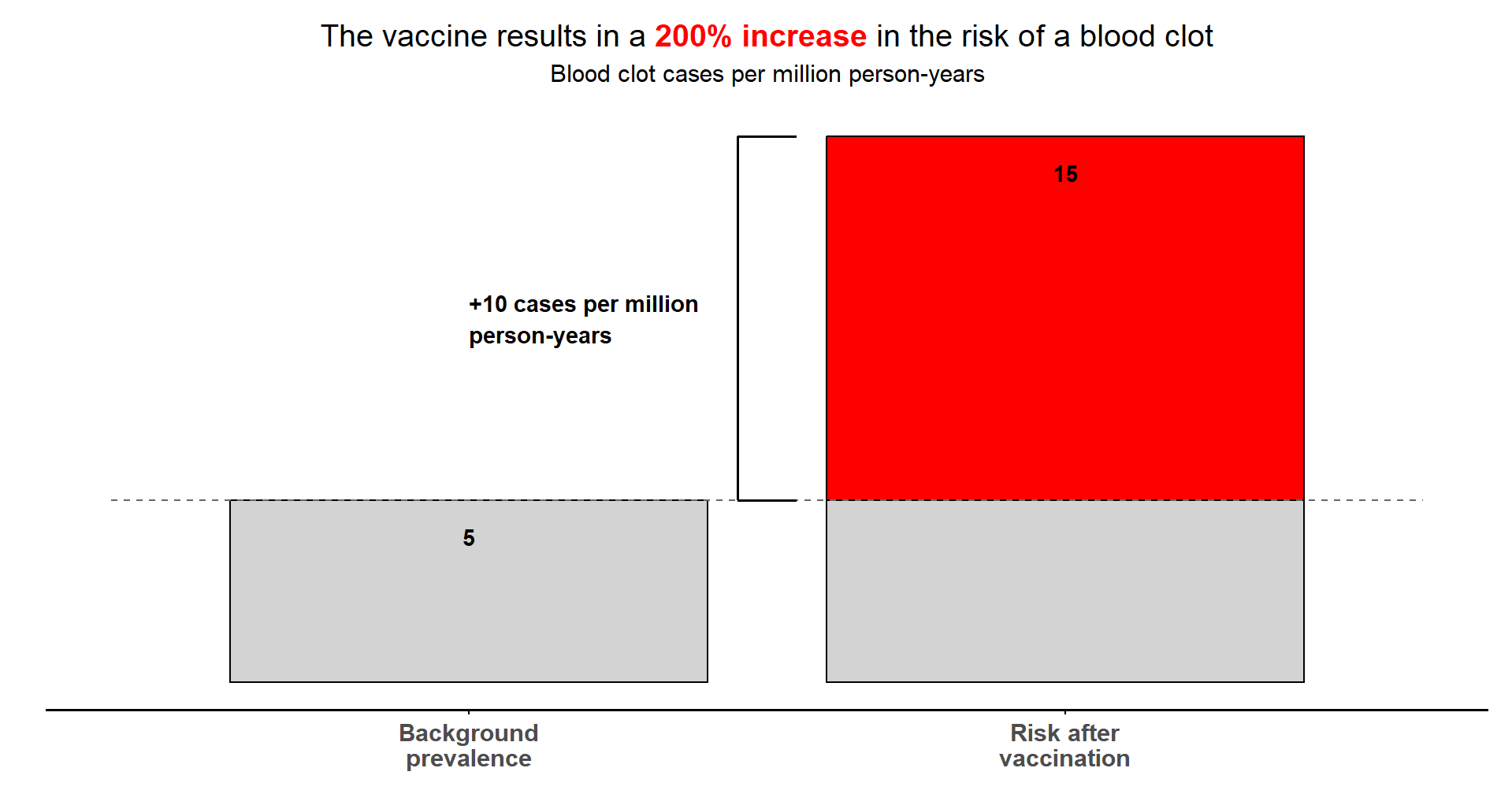
- Background CVST prevalence: 5 cases per million person-years
- CVST attributable to vaccine: 10 additional cases per million person-years
Challenge #1
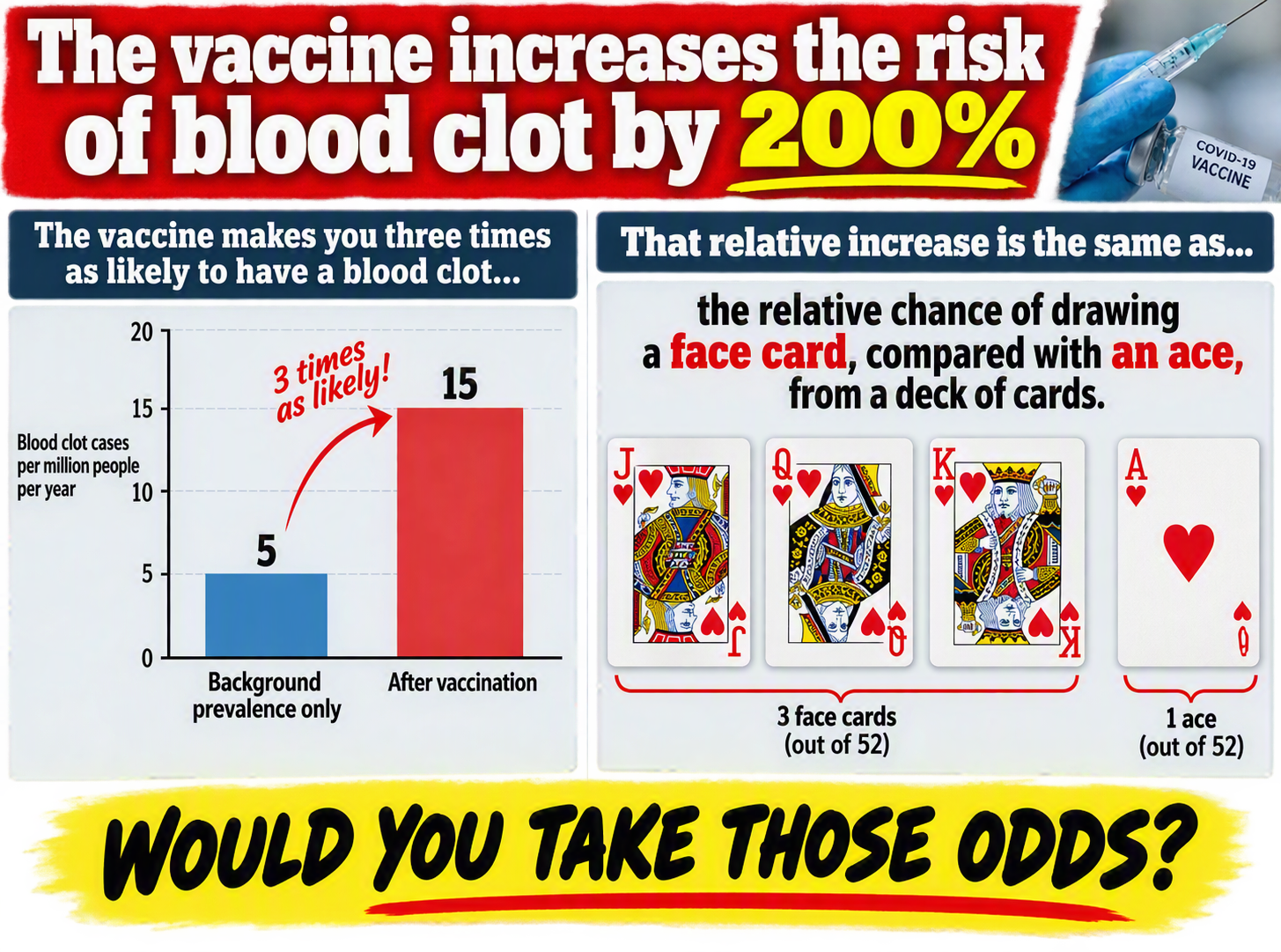
You are a journalist working on a tabloid newspaper. Produce an eye-catching and dramatic visualisation emphasising the dangers of vaccination, based on relative risk (200% increase in blood clot risk!).
Challenge #2
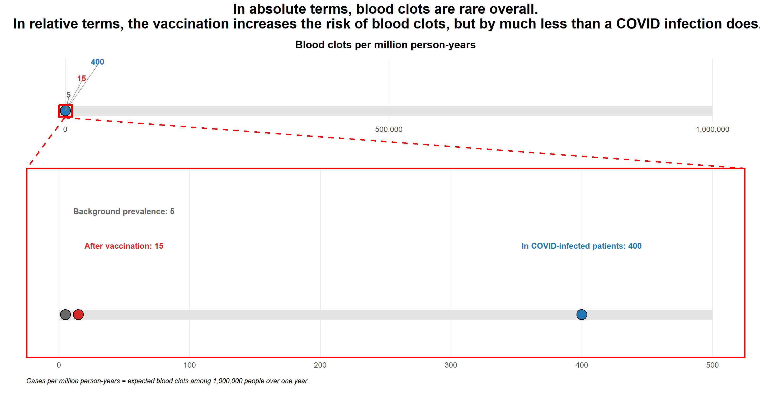
You work for a medical communications agency, educating healthcare providers and the public on vaccine benefits and risks. Produce an alternative visualisation showing CVST risk of the vaccine on an absolute scale e.g. comparing absolute risks or number needed to harm (NNH).
Do you draw a different conclusion?
Some more assumptions:
- COVID infection rate (without vaccine protection): 30%
- CVST prevalence in COVID-infected patients: 400 cases*
- Vaccine effectiveness: 70%
Challenge #3
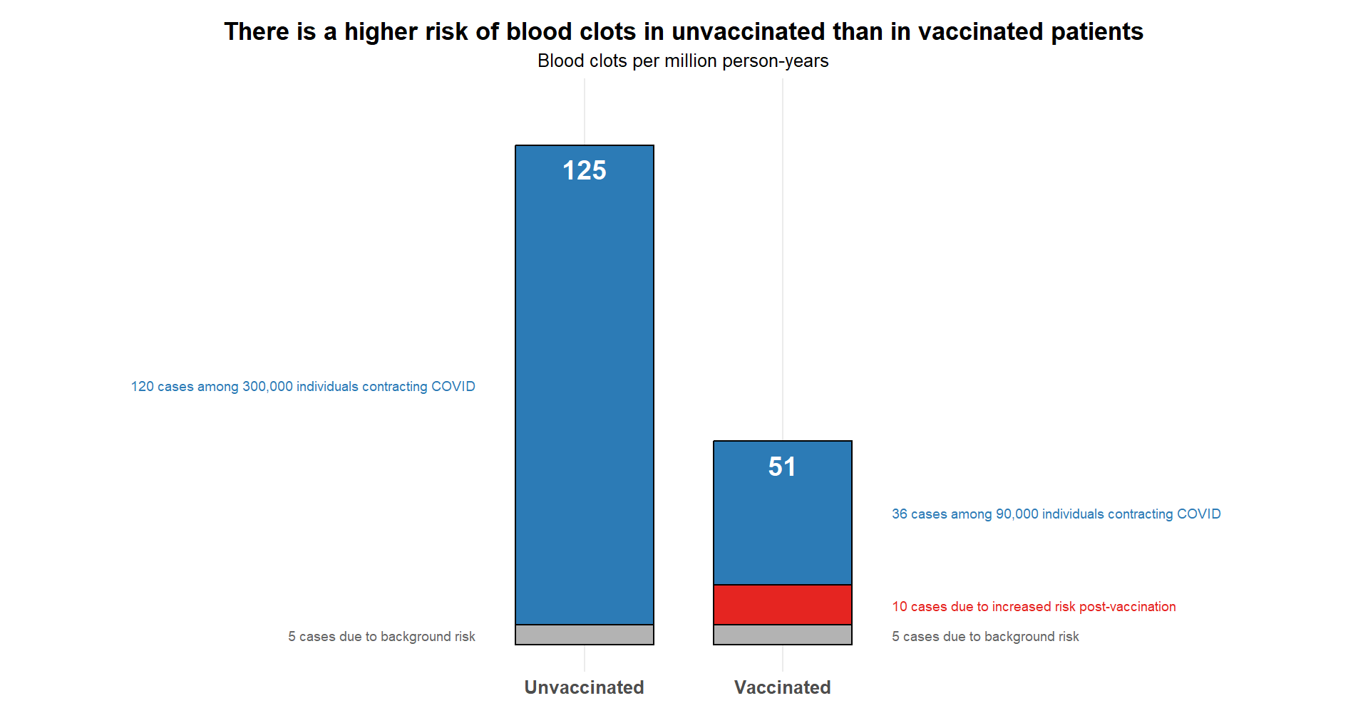
Produce a visualisation communicating the true risk of CVST. Compare CVST prevalence in vaccinated patients (approx. 46 cases) to unvaccinated patients (approx. 120 cases), after accounting for the CVST rate in COVID patients.
Challenge #4 (Bonus)
Produce a visualisation from a tipping point analysis: What is the minimum vaccine side effect (CVST additional cases attributable to the vaccine*) at which point the vaccine is worse than unvaccinated patients?
’* Per million person-years
Visualisations
Submission 1, Challenge 1
Submission 2, Challenge 1
Submission 2, Challenge 2/3
Submission 2, Challenge 3
Submission 3, All Challenges

Submission 3 is an interactive app that addresses all of the challenges as you work through it. Visit and explore the app here.
Code
Code for Submission 2, Challenge 1
# Load Required Packages
library(ggplot2)
library(ggtext)
library(grid)

# Risk Values
background_risk <- 5
total_risk <- 15
additional_risk <- total_risk - background_risk

#Create Plot
ggplot() +

  # Background prevalence bar
  geom_rect(
    aes(
      xmin = 0.6,
      xmax = 1.4,
      ymin = 0,
      ymax = background_risk
    ),
    fill = "light grey",
    colour = "black"
  ) +

  # Grey section of vaccination bar
  geom_rect(
    aes(
      xmin = 1.6,
      xmax = 2.4,
      ymin = 0,
      ymax = background_risk
    ),
    fill = "light grey",
    colour = "black"
  ) +

  # Additional risk section of vaccination bar
  geom_rect(
    aes(
      xmin = 1.6,
      xmax = 2.4,
      ymin = background_risk,
      ymax = total_risk
    ),
    fill = "red",
    colour = "black"
  ) +

  # Dashed line showing background prevalence level
  geom_segment(
    aes(x = 0.4, xend = 2.6,
        y = background_risk, yend = background_risk),
    linetype = "dashed",
    colour = "grey40",
    linewidth = 0.8
  ) +

  # Value labels inside bars
  annotate(
    "text",
    x = 1,
    y = background_risk - 1,
    label = background_risk,
    fontface = "bold",
    size = 7
  ) +

  annotate(
    "text",
    x = 2,
    y = total_risk - 1,
    label = total_risk,
    fontface = "bold",
    size = 7
  ) +

  # Annotation showing additional risk
  annotate(
    "segment",
    x = 1.45, xend = 1.45,
    y = background_risk, yend = total_risk,
    linewidth = 1
  ) +

  annotate(
    "segment",
    x = 1.45, xend = 1.55,
    y = background_risk, yend = background_risk,
    linewidth = 1
  ) +

  annotate(
    "segment",
    x = 1.45, xend = 1.55,
    y = total_risk, yend = total_risk,
    linewidth = 1
  ) +

  annotate(
    "text",
    x = 1,
    y = background_risk + 0.5*additional_risk,
    label = paste0("+", additional_risk,
                   " cases per million\nperson-years"),
    hjust = 0,
    fontface = "bold",
    size = 7
  ) +

  scale_x_continuous(
    breaks = c(1, 2),
    labels = c(
      "Background\nprevalence",
      "Risk after\nvaccination"
    )
  ) +

  labs(
    title = paste0(
      "The vaccine results in a ",
      "<span style='color:", "red", ";'><b>200% increase</b></span>",
      " in the risk of a blood clot"
    ),
    subtitle = "Blood clot cases per million person-years"
  ) +

  theme_minimal(base_size = 16) +

  theme(
    plot.title = element_markdown(
      size = 27,
      face = "plain",
      hjust = 0.5,
      margin = margin(b = 10)
    ),

    plot.subtitle = element_text(
      size = 21,
      hjust = 0.5,
      margin = margin(b = 20)
    ),

    # Remove all y-axis elements
    axis.title.y = element_blank(),
    axis.text.y = element_blank(),
    axis.ticks.y = element_blank(),
    panel.grid.major.y = element_blank(),
    panel.grid.minor = element_blank(),

    # Keep prominent x-axis
    axis.title.x = element_blank(),
    axis.line.x = element_line(
      colour = "black",
      linewidth = 1.2
    ),
    axis.ticks.x = element_line(
      colour = "black"
    ),

    axis.text.x = element_text(
      size = 21,
      face = "bold"
    ),

    panel.grid.major.x = element_blank(),

    axis.line.y = element_blank(),

    plot.margin = margin(
      t = 20,
      r = 20,
      b = 20,
      l = 40
    )
  )
Code for Submission 2, Challenge 2/3
# Load Required Packages
library(ggplot2)
library(patchwork)
library(scales)
library(cowplot)

# Risk Values
background_risk <- 5
total_risk <- 15
covid_risk <- 400

risk_data <- data.frame(
  label = c(
    paste("Background prevalence:", background_risk),
    paste("After vaccination:", total_risk),
    paste("In COVID-infected patients:", covid_risk)
  ),
  risk = c(background_risk, total_risk, covid_risk),
  colour = c("grey40", "#d62828", "#1f77b4"),

  # Label positions for top panel
  label_x = c(50, 50, covid_risk),
  label_y = c(1.15, 1.1, 1.1)
)

# Labels for lower panel
lower_labels <- data.frame(
  risk = c(background_risk, total_risk, covid_risk),
  label_x = c(5000, 25000, 50000),
  y = c(1.1, 1.2, 1.3),
  label = c(paste(background_risk),
            paste(total_risk),
            paste(covid_risk)),
  colour = c("grey40", "#d62828", "#1f77b4")
)

# Top Panel
p_main <- ggplot(risk_data) +

  annotate(
    "segment",
    x = 0,
    xend = 1.25*covid_risk,
    y = 1,
    yend = 1,
    linewidth = 8,
    colour = "grey90"
  ) +

  geom_point(
    aes(
      x = risk,
      y = 1,
      fill = colour
    ),
    shape = 21,
    size = 8,
    colour = "black",
  ) +

  scale_fill_identity() +

  geom_text(
    aes(
      x = label_x,
      y = label_y,
      label = label,
      colour = colour
    ),
    fontface = "bold",
    size = 5
  ) +

  scale_colour_identity() +

  scale_x_continuous(
    limits = c(0, 500),
    breaks = seq(0, 500, 100)
  ) +

  coord_cartesian(
    ylim = c(0.95, 1.2),
  ) +

  labs(
    caption = paste("Cases per million person-years = expected blood clots",
                    "among 1,000,000 people over one year.")
  ) +

  theme_minimal(base_size = 16) +

  theme(
    axis.title = element_blank(),
    axis.text.y = element_blank(),
    axis.ticks.y = element_blank(),
    plot.title = element_blank(),

    panel.border = element_rect(
      colour = "red",
      fill = NA,
      linewidth = 2
    ),

    panel.grid.major.y = element_blank(),
    panel.grid.minor = element_blank(),

    plot.caption = element_text(
      hjust = 0,
      face = "italic",
      size = 12,
      margin = margin(t = 15)
    ),

    plot.margin = margin(
      t = 40,
      r = 20,
      b = 20,
      l = 40
    )
  )

# Bottom Panel
p_inset <- ggplot(risk_data) +

  annotate(
    "segment",
    x = 0,
    xend = 1000000,
    y = 1,
    yend = 1,
    linewidth = 8,
    colour = "grey90"
  ) +

  geom_point(
    aes(
      x = risk,
      y = 1,
      fill = colour
    ),
    shape = 21,
    size = 8,
    colour = "black"
  ) +

  # Leader lines from labels to points
  geom_segment(
    data = lower_labels,
    aes(
      x = risk,
      xend = label_x,
      y = 1,
      yend = y - 0.02
    ),
    colour = "grey50",
    linewidth = 0.5
  ) +

  # Labels
  geom_text(
    data = lower_labels,
    aes(
      x = label_x,
      y = y,
      label = label,
      colour = colour
    ),
    fontface = "bold",
    size = 5
  ) +

  scale_fill_identity() +
  scale_colour_identity() +

  scale_x_continuous(
    limits = c(-10000, 1000000),
    breaks = c(0, 500000, 1000000),
    labels = comma
  ) +

  coord_cartesian(
    ylim = c(0.95, 1.3),
  ) +

  labs(
    title = paste("Blood clots per million person-years"),
  ) +

  theme_minimal(base_size = 16) +

  annotate(
    "rect",
    xmin = -10000,
    xmax = 10000,
    ymin = 0.965,
    ymax = 1.035,
    colour = "red",
    fill = NA,
    linewidth = 1.5
  ) +

  theme(
    axis.title = element_blank(),
    axis.text.y = element_blank(),
    axis.ticks.y = element_blank(),

    panel.grid.major.y = element_blank(),
    panel.grid.minor = element_blank(),

    plot.title = element_text(
      hjust = 0.5,
      face = "bold",
      size = 18,
      margin = margin(b = 15)
    ),

    plot.margin = margin(
      t = 10,
      r = 20,
      b = 20,
      l = 20
    )
  )

# Combined Plot
combined_plot <-
(p_inset / p_main) +
  plot_layout(
    heights = c(1, 3)
  ) +
  plot_annotation(
    title = paste("In absolute terms, blood clots are rare overall.\n",
                  "In relative terms, the vaccination increases the risk",
                  "of blood clots, but by much less than",
                  "a COVID infection does."),
    theme = theme(
      plot.title = element_text(
        hjust = 0.5,
        size = 24,
        face = "bold"
      )
    )
  )

# Drawing connecting lines for zoom effect
# NOTE - VALUES MANUALLY TOGGLED TO LINE UP NICELY IN ZOOMED WINDOW
# WILL NOT ALWAYS LINE UP AS DESIRED
ggdraw(combined_plot) +

  draw_line(
    x = c(0.085, 0.035),
    y = c(0.705, 0.577),
    colour = "red",
    linetype = "dashed",
    linewidth = 1.2
  ) +

  draw_line(
    x = c(0.085, 0.98),
    y = c(0.705, 0.578),
    colour = "red",
    linetype = "dashed",
    linewidth = 1.2
  )
Code for Submission 2, Challenge 3
# Load Required Packages
library(ggplot2)
library(ggtext)

# Data Setup
background_cases <- 5
vaccine_cases <- 10
covid_infections_vaccinated <- 0.3*(1-0.7)*1000000
covid_infections_unvaccinated <- 0.3*1000000
covid_cases_vaccinated <- 0.3*(1-0.7)*400
covid_cases_unvaccinated <- 0.3*400

plot_data <- data.frame(
  group = rep(c("Unvaccinated", "Vaccinated"), each = 3),
  component = c(
    "Background", "Vaccine", "COVID",
    "Background", "Vaccine", "COVID"
  ),
  value = c(
    background_cases, 0, covid_cases_unvaccinated,
    background_cases, vaccine_cases, covid_cases_vaccinated
  )
)

plot_data$component <- factor(
  plot_data$component,
  levels = c("COVID", "Vaccine", "Background")
)

totals <- aggregate(
  value ~ group,
  data = plot_data,
  sum
)

# Annotations
annot_data <- data.frame(
  x = c(
    0.45,  # unvaccinated background
    0.45,  # unvaccinated covid

    2.55,  # vaccinated background
    2.55,  # vaccinated vaccine
    2.55   # vaccinated covid
  ),

  y = c(
    background_cases/2,
    background_cases + covid_cases_unvaccinated/2,

    background_cases/2,
    background_cases + vaccine_cases/2,
    background_cases + vaccine_cases + covid_cases_vaccinated/2
  ),

  label = c(
    paste(background_cases,
          "cases due to background risk"),

    paste(covid_cases_unvaccinated,
          "cases among",
          format(covid_infections_unvaccinated,
                 big.mark = ",", scientific = FALSE),
          "individuals contracting COVID"),

    paste(background_cases,
          "cases due to background risk"),

    paste(vaccine_cases,
          "cases due to increased risk post-vaccination"),

    paste(covid_cases_vaccinated,
          "cases among",
          format(covid_infections_vaccinated,
                 big.mark = ",", scientific = FALSE),
          "individuals contracting COVID")
  ),

  colour = c(
    "grey40",
    "#2c7bb6",

    "grey40",
    "#e52521",
    "#2c7bb6"
  )
)

# Plot
ggplot(
  plot_data,
  aes(
    x = group,
    y = value,
    fill = component
  )
) +

  geom_col(
    width = 0.7,
    colour = "black",
    linewidth = 0.8
  ) +

  scale_fill_manual(
    values = c(
      "Background" = "grey70",
      "Vaccine"    = "#e52521",
      "COVID"      = "#2c7bb6"
    )
  ) +

geom_text(
  data = totals,
  aes(
    x = group,
    y = value - 6,
    label = value
  ),
  inherit.aes = FALSE,
  colour = "white",
  fontface = "bold",
  size = 9
) +

  geom_text(
    data = subset(annot_data, x < 1),
    aes(
      x = x,
      y = y,
      label = label,
      colour = colour
    ),
    inherit.aes = FALSE,
    hjust = 1,
    size = 4.5
  ) +

  geom_text(
    data = subset(annot_data, x > 1),
    aes(
      x = x,
      y = y,
      label = label,
      colour = colour
    ),
    inherit.aes = FALSE,
    hjust = 0,
    size = 4.5
  ) +

  scale_colour_identity() +

  labs(
    title = paste("There is a higher risk of blood clots in unvaccinated",
                  "than in vaccinated patients"),
    subtitle = "Blood clots per million person-years",
    x = NULL,
    y = NULL
  ) +

  coord_cartesian(
    xlim = c(-0.2, 3.2),
    ylim = c(0, max(totals$value)+10),
    clip = "off"
  ) +

  theme_minimal(base_size = 16) +

  theme(
    plot.title = element_text(
      hjust = 0.5,
      face = "bold",
      size = 24
    ),

    plot.subtitle = element_text(
      hjust = 0.5,
      size = 18
    ),

    axis.text.x = element_text(
      size = 18,
      face = "bold"
    ),

    axis.title = element_blank(),
    axis.text.y = element_blank(),
    axis.ticks.y = element_blank(),

    panel.grid.major.y = element_blank(),
    panel.grid.minor = element_blank(),

    legend.position = "none",

    plot.margin = margin(
      t = 20,
      r = 220,
      b = 20,
      l = 220
    )
  )