Protocol Amendment Storytelling
Note: this is the challenge that was set during the July 2026 webinar. There was no webinar in August 2026.
Background
There is a hypothetical Phase III clinical trial for a chronic disease. During study conduct, recruitment is slower than anticipated. A major protocol amendment is introduced at Month 10 to relax eligibility criteria, reduce visit frequency and simplify data collection requirements.
The Challenge
The sponsor would like to understand whether the amendment successfully improved trial performance.
Create a data visualisation that clearly communicates any of the following (or any other ‘story’ you find interesting to convey to the sponsor):
- What changed after the amendment
- Whether recruitment improved
- Whether operational efficiency improved
- Any trade-offs or unintended consequences
The Data
24 months of study conduct (amendment introduced at Month 10). The dataset includes the following variables:
| Variable Name | Variable Label |
|---|---|
| Month | Study month (1-24) |
| Amendment_Status | Before/After Amendment (indicator) |
| New_Subjects_Enrolled | Number of subjects enrolled during the month |
| Screen_Failure_Rate | Percentage of screened subjects failing eligibility criteria |
| Active_Sites | Number of sites actively recruiting |
| Protocol_Deviations | Number of protocol deviations recorded |
| Avg_Query_Days | Average time (days) to resolve data queries |
| Avg_Visit_Burden | Mean scheduled visits per patient |
| Retention_Rate | Percentage of randomised subjects remaining in follow-up |
| Monitoring_Cost_GBP | Estimated monitoring expenditure (£) |
Visualisations
Submission 1: Sponsor Report
Submission 1 is a full sponsor report. Hence, it is best viewed via the HTML file.
View the HTML file: Sponsor Report
Submission 2: Bar Chart

Code
Code for Submission 1
---
title: "Impact of Protocol Amendment - Sponsor Report"
subtitle: "PSI Wonderful Wednesday Visualisation Challenge - September 2026"
format:
  html:
    toc: true
    toc-depth: 2
    code-fold: true
    theme: cosmo
    highlight-style: github
execute:
  echo: false
  warning: false
  message: false
---

## Executive Summary

This report evaluates the impact of a clinical trial protocol amendment for a sponsor. During study conduct of a hypothetical Phase III clinical trial for a chronic disease, recruitment is slower than anticipated. A major protocol amendment is introduced at Month 10 to relax eligibility criteria, reduce visit frequency and simplify data collection requirements.
The report focuses on three critical dimensions of trial performance: **enrollment**, **quality**, and **costs**. Our analysis compares metrics before the amendment (Months 1-9) and after the amendment (Months 10+) to determine whether the amendment successfully improved trial operations.

## Background

The protocol amendment represents a significant operational change to the clinical trial. By comparing key performance indicators before and after Month 10, we can assess whether the amendment achieved its intended objectives and check for any unintended consequences on trial operations.

## Data and Methods

```{r}
#| label: setup
library(tidyverse)
library(ggplot2)
library(readxl)
library(gridExtra)

# Load data
df <- read_excel("Protocol Amendment Dataset.xlsx", sheet = 1)

# Create derived variables
df <- df |>
  mutate(
    Total_Enrollments = cumsum(New_Subjects_Enrolled),
    Dev_per_subject = Protocol_Deviations / Total_Enrollments,
    new_enr_per_site = New_Subjects_Enrolled / Active_Sites
  )

# Define plot variables and labels
plot_vars <- list(
  New_Subjects_Enrolled = "New Subjects Enrolled",
  new_enr_per_site = "New Subjects Enrolled per Site",
  Screen_Failure_Rate = "Screen Failure Rate (%)",
  Active_Sites = "Active Sites",
  Protocol_Deviations = "Protocol Deviations",
  Dev_per_subject = "Deviations per Subject",
  Avg_Query_Days = "Average Query Days",
  Avg_Visit_Burden = "Scheduled visits per patient",
  Retention_Rate = "Retention Rate (%)",
  Monitoring_Cost_GBP = "Monitoring Cost (GBP)"
)

# Create summary means table
summary_means <- df |>
  mutate(Period = if_else(Month < 10, "Before", "After")) |>
  select(Month, Period, all_of(names(plot_vars))) |>
  pivot_longer(
    cols = -c(Month, Period),
    names_to = "Metric",
    values_to = "Value"
  ) |>
  group_by(Period, Metric) |>
  summarise(Mean = mean(Value, na.rm = TRUE), .groups = "drop") |>
  pivot_wider(names_from = Period, values_from = Mean) |>
  mutate(
    Metric = factor(Metric, levels = names(plot_vars)),
    Metric_Label = sapply(as.character(Metric), function(x) plot_vars[[x]]),
    Change = After - Before,
    Pct_Change = round((Change / Before) * 100, 1)
  )

# Function to create before/after plot
create_before_after_plot <- function(metric_name,ndec) {
  metric_data <- summary_means |>
    filter(Metric == metric_name) |>
    pivot_longer(cols = c(Before, After), names_to = "Period", values_to = "Mean_Value")

  metric_label <- plot_vars[[metric_name]]

  plot <- ggplot(metric_data, aes(x = Period, y = Mean_Value, fill = Period)) +
    geom_col(alpha = 0.8, width = 0.6) +
    geom_text(aes(label = format(round(Mean_Value, ndec), nsmall = 1)),
              vjust = -0.5, size = 4, fontface = "bold") +
    scale_fill_manual(values = c("Before" = "steelblue", "After" = "darkgreen")) +
    scale_x_discrete(limits = c("Before", "After")) +
    labs(
      title = metric_label,
      x = "Period",
      y = "Mean Value"
    ) +
    theme_minimal() +
    theme(
      plot.title = element_text(size = 11, face = "bold"),
      axis.title = element_text(size = 10),
      axis.text.x = element_text(face = "bold", size = 10),
      legend.position = "none"
    )

  return(plot)
}
```

Data was analyzed by comparing mean values of key performance indicators in two periods: **Before Amendment** (Months 1-9, n=9 months) and **After Amendment** (Months 10+, n=15 months). The protocol amendment was implemented at the beginning of Month 10.

---

## Results

### 1. Enrollment Metrics

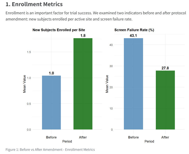
Enrollment is an important factor for trial success. We examined two indicators before and after protocol amendment: new subjects enrolled per active site and screen failure rate.

```{r}
#| label: fig-enrollment
#| fig-cap: "Before vs After Amendment - Enrollment Metrics"

e1 <- create_before_after_plot("new_enr_per_site", ndec = 1)
e2 <- create_before_after_plot("Screen_Failure_Rate", ndec = 1)

grid.arrange(e1, e2, ncol = 2)

```

**Key Findings:**

- **New Subjects Enrolled**: The amendment resulted in an increase in the average number of new subjects enrolled per site.

- **Screen failure rate**: The average screen failure rate dropped after the protocol amendment.

These findings suggest that the amendment improved trial enrollment.

---

### 2. Quality Metrics

Trial quality reflects adherence to protocol and data quality. We examined protocol deviations per subject, average query resolution time and retention rate.

```{r}
#| label: fig-quality
#| fig-cap: "Before vs After Amendment - Quality Metrics"

q1 <- create_before_after_plot("Dev_per_subject",ndec = 2)
q2 <- create_before_after_plot("Avg_Query_Days",ndec = 1)
q3 <- create_before_after_plot("Retention_Rate",ndec = 1)

grid.arrange(q1, q2,q3, ncol = 3)
```

**Key Findings:**


- **Deviations per Subject**: Per-subject deviation rate decreased after the protocol amendment, reflecting the quality impact adjusted for enrollment volume.

- **Average Query Days**: Query resolution time decreased after protocol amendment.

- **Retention rate**: The average retention rate was similar in the months before and after protocol amendment.

These findings indicate that the amendment improved trial integrity and data quality.

---

### 3. Cost Metrics

Trial efficiency also depends on managing operational costs and trial participant burden. We examined monitoring costs and visit burden.

```{r}
#| label: fig-costs
#| fig-cap: "Before vs After Amendment - Cost and Burden Metrics"

c1 <- create_before_after_plot("Monitoring_Cost_GBP",ndec = 0)
c2 <- create_before_after_plot("Avg_Visit_Burden", ndec = 1)

grid.arrange(c1,c2, ncol = 2)

```

**Key Findings:**

- **Monitoring Costs**: Average monitoring costs decreased slightly after protocol amendment.
- **Visit burden**: The visit burden decreased after protocol amendment.

These findings show a positive effect on visit burden for trial participants after the protocol amendment. While the monitoring costs decreased only slightly after protocol amendment, the costs might also have been impacted by increased enrollment numbers after the amendment.

---

## Conclusion

The protocol amendment represented a substantive operational change to the clinical trial.
Enrollment data shows a positive trend in participant recruitment following the amendment. Quality metrics also show improved data quality and integrity after the amendment. Further analysis could be performed to better understand the impact on monitoring costs.
No unintended consequences on trial operations were identified from this analysis.
The analysis results indicate that the protocol amendment was successful in improving trial performance.

---
Code for Submission 2
#=================================================
# Load Required Packages
#=================================================
library(readxl)
library(dplyr)
library(ggplot2)
library(grid)


#=================================================
# Import Data
#=================================================
dat <- read_excel("Protocol Amendment Dataset.xlsx")

#=================================================
# Plot
#=================================================
ggplot(
  dat,
  aes(
    x = Month,
    y = New_Subjects_Enrolled,
    fill = Amendment_Status
  )
) +
  geom_col() +
  geom_text(
    aes(label = New_Subjects_Enrolled,
        colour = Amendment_Status),
    vjust = -0.25,
    size = 5
  ) +
  annotate(
    "segment",
    x = 9.5,
    xend = 9.5,
    y = 0,
    yend = max(dat$New_Subjects_Enrolled) + 3,
    colour = "#D55E00",
    linewidth = 1.2,
    linetype = 2
  ) +
  annotate(
    "text",
    x = 9.5,
    y = max(dat$New_Subjects_Enrolled) + 5,
    label = "Protocol amendment introduced",
    colour = "#D55E00",
    size = 6
  ) +
  annotate(
    "text",
    x = 5,
    y = max(dat$New_Subjects_Enrolled) + 5,
    label = "Pre-Amendment",
    colour = "grey55",
    size = 6
  ) +
  annotate(
    "text",
    x = 17,
    y = max(dat$New_Subjects_Enrolled) + 5,
    label = "Post-Amendment",
    colour = "#4EA5D9",
    size = 6
  ) +
  scale_fill_manual(
    values = c(
      "Before Amendment" = "grey55",
      "After Amendment" = "#4EA5D9"
    )
  ) +
  scale_colour_manual(
    values = c(
      "Before Amendment" = "grey55",
      "After Amendment" = "#4EA5D9"
    )
  ) +
  scale_x_continuous(
    breaks = 1:24,
    expand = expansion(mult = c(0, 0))
  ) +

  scale_y_continuous(
    expand = expansion(mult = c(0, 0.05))
  ) +
  labs(
    title = "Monthly Enrolment",
    subtitle = paste("Enrolment increased immediately following the amendment",
                     "and continued to rise throughout the remainder",
                     "of the study")
  ) +
  theme_minimal() +
  theme(
    axis.title.y = element_blank(),
    axis.text.y = element_blank(),
    axis.ticks.y = element_blank(),
    panel.grid.major = element_blank(),
    panel.grid.minor = element_blank(),
    axis.title.x = element_text(size = 18),
    axis.text.x = element_text(size = 12),
    axis.line.x = element_line(colour = "black", size = 2),
    legend.position = "none",
    plot.title = element_text(
      face = "bold",
      size = 30,
      hjust = 0.5,
      margin = margin(
        b = 15
      )
    ),
    plot.subtitle = element_text(
      size = 20,
      hjust = 0.5,
      margin = margin(
        b = 35
      )
    ),
    plot.margin = margin(
      t = 25,
      r = 25,
      b = 20,
      l = 25
    )
  )