Make Better Choices
The background
There is a recent publication: Behavior change intervention targeting physical activity and diet improves stress and sleep.
It describes the results of the Make better choices 2 trial.
The publication is available via PubMed.
The challenge
The challenge is to find or create a better or more suitable plot than the ones provided in the publication.
Fig 1. Predicted average daily stress (+/-95% CI) across time as a function of intervention type
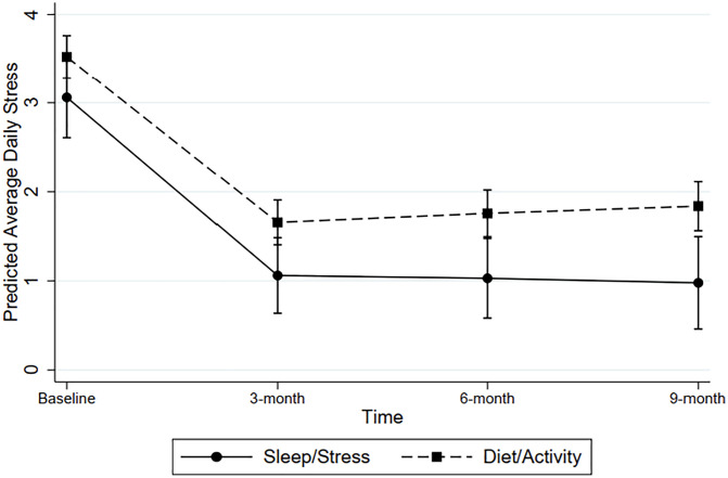
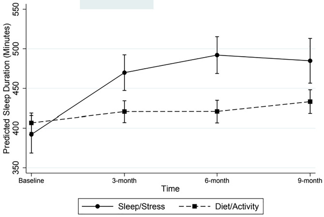
Fig 2. Predicted Mean (+/-95% CI) Sleep Duration Across Time as a Function of Intervention Type
Visualisations
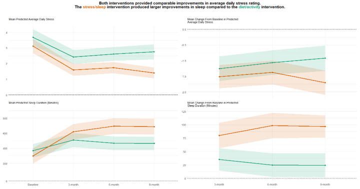
Example 1: Static Lineplots (1)
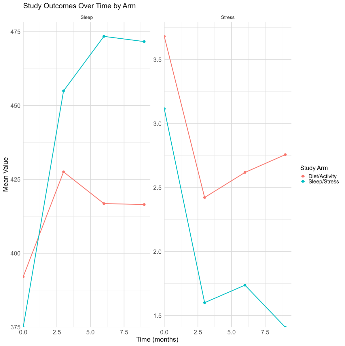
Example 2: Static Lineplots (2)
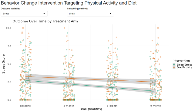
Example 3: Dashboard
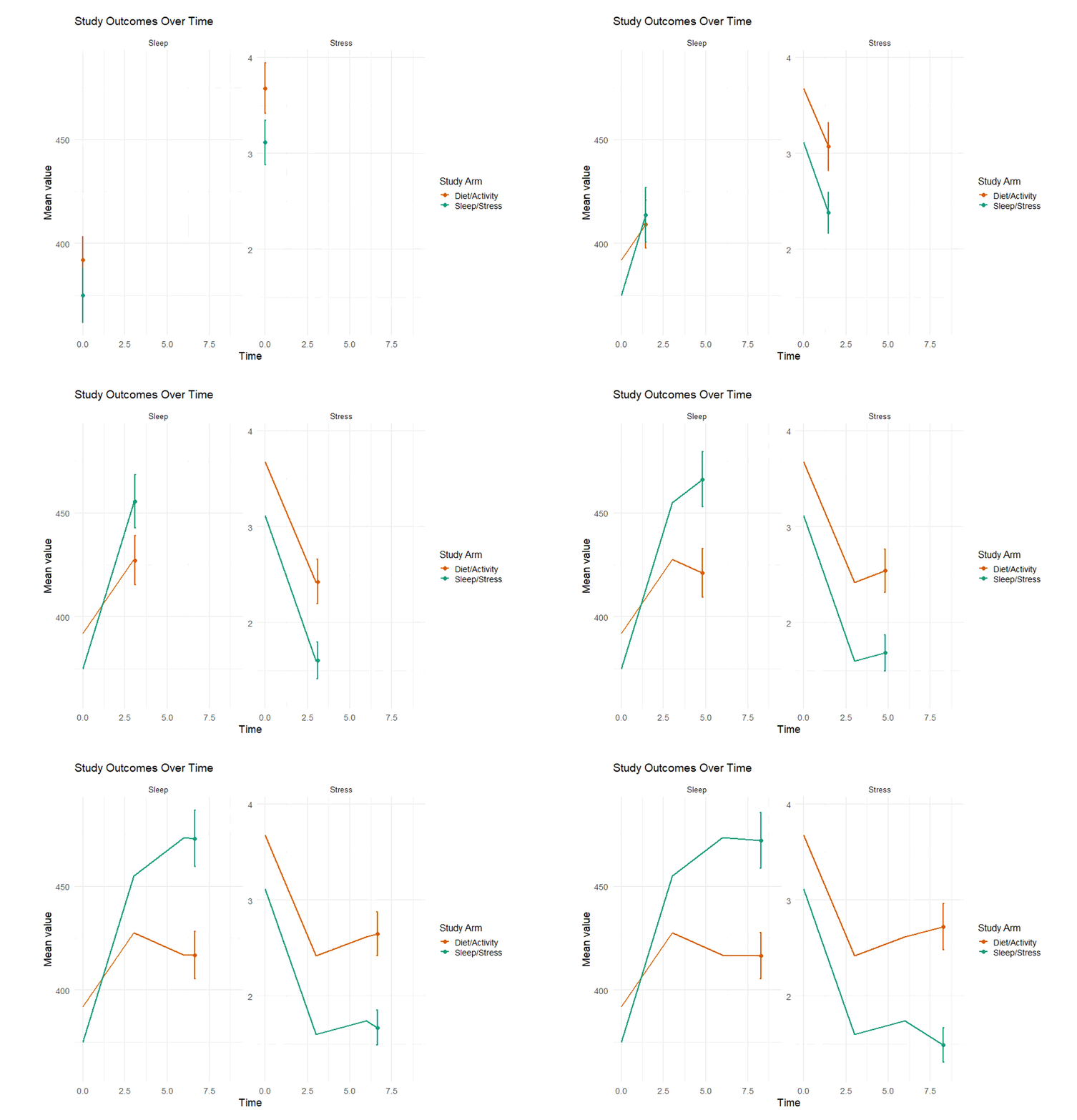
Example 4: Animated Lineplot
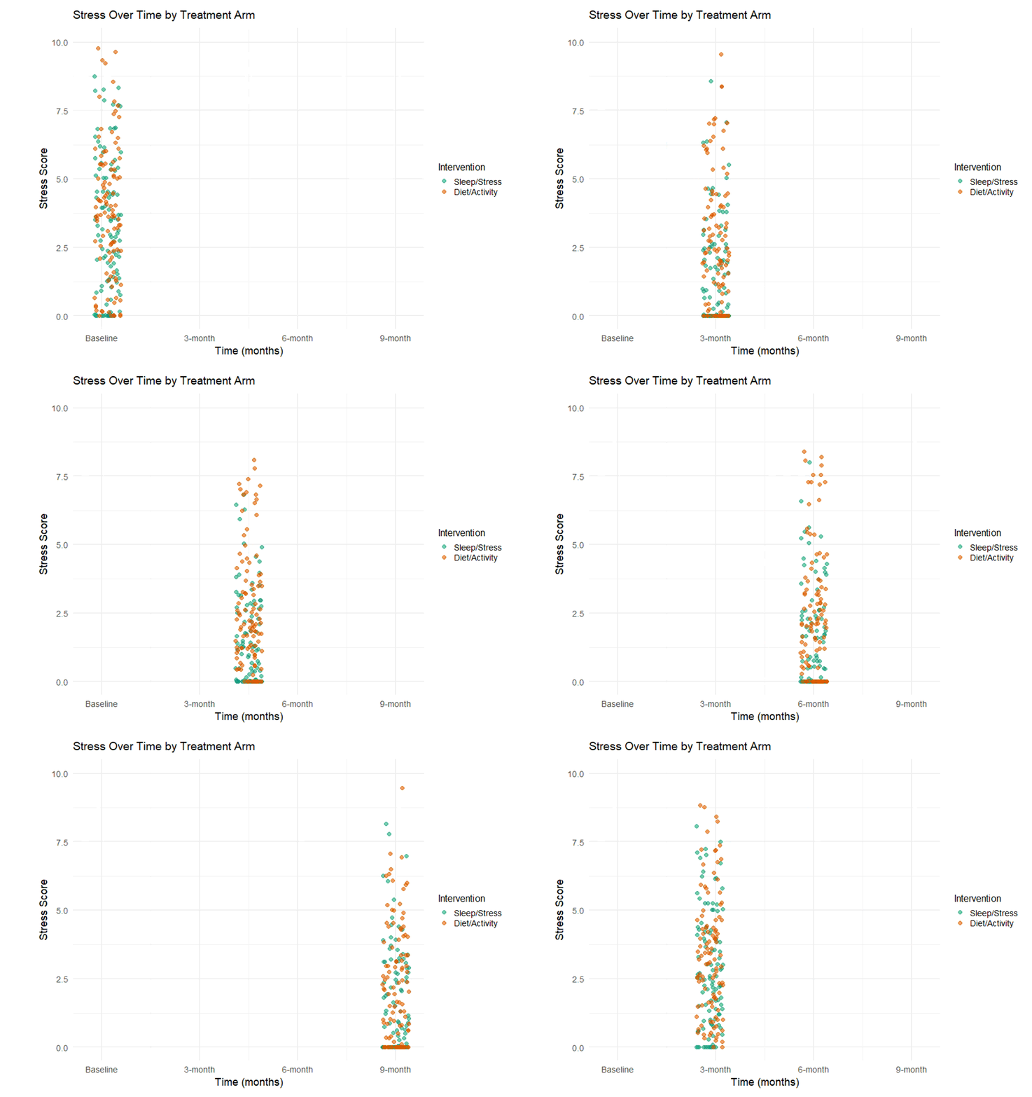
Example 5: Animated Scatter Plot
Code
Code for Example 1
# Load Required Packages
library(readr)
library(tidyverse)
library(ggplot2)
library(patchwork)
library(ggbreak)
library(ggtext)

# Load Data
df_pre <- read_csv("simulated_MBC2_data.csv")

# Derive CFB for Post-BL Visits
df_bl <- df_pre %>%
  filter(time_f == 'Baseline') %>%
  select(id, stress, sleep) %>%
  rename(stress_bl = stress,
         sleep_bl = sleep)

df_all <- df_pre %>%
  left_join(df_bl, by = "id") %>%
  mutate(stress_chg = if_else(time_f != 'Baseline',
                              stress - stress_bl,
                              NA_real_),
         sleep_chg = if_else(time_f != 'Baseline',
                             sleep - sleep_bl,
                             NA_real_))

# Deriving Mean and CIs for AVALs and CHGs by TRT and Visit
df <- df_all %>%
  group_by(arm, time_f) %>%
  summarise(

    stress_mean = mean(stress, na.rm = TRUE),
    stress_low  = mean(stress, na.rm = TRUE) - 1.96 * sd(stress, na.rm = TRUE)/sqrt(sum(!is.na(stress))),
    stress_high  = mean(stress, na.rm = TRUE) + 1.96 * sd(stress, na.rm = TRUE)/sqrt(sum(!is.na(stress))),

    stress_chg_mean = mean(stress_chg, na.rm = TRUE),
    stress_chg_low  = mean(stress_chg, na.rm = TRUE) - 1.96 * sd(stress_chg, na.rm = TRUE)/sqrt(sum(!is.na(stress_chg))),
    stress_chg_high  = mean(stress_chg, na.rm = TRUE) + 1.96 * sd(stress_chg, na.rm = TRUE)/sqrt(sum(!is.na(stress_chg))),

    sleep_mean = mean(sleep, na.rm = TRUE),
    sleep_low  = mean(sleep, na.rm = TRUE) - 1.96 * sd(sleep, na.rm = TRUE)/sqrt(sum(!is.na(sleep))),
    sleep_high  = mean(sleep, na.rm = TRUE) + 1.96 * sd(sleep, na.rm = TRUE)/sqrt(sum(!is.na(sleep))),

    sleep_chg_mean = mean(sleep_chg, na.rm = TRUE),
    sleep_chg_low  = mean(sleep_chg, na.rm = TRUE) - 1.96 * sd(sleep_chg, na.rm = TRUE)/sqrt(sum(!is.na(sleep_chg))),
    sleep_chg_high  = mean(sleep_chg, na.rm = TRUE) + 1.96 * sd(sleep_chg, na.rm = TRUE)/sqrt(sum(!is.na(sleep_chg)))

    )

###################################################################
# Plot Code Generated Using CoPilot
# NOT REVIEWED AT LENGTH - SHOULD UNDERGO HUMAN REVIEW BEFORE REUSE
###################################################################
df$time_f <- factor(
  df$time_f,
  levels = c("Baseline", "3-month", "6-month", "9-month")
)

# ----------------------------
# Define colours
# ----------------------------
col_da <- "#1B9E77"   # Diet/Activity
col_ss <- "#D95F02"   # Sleep/Stress

# -----------------------------------------------------
# Helper plotting function (NO y-axis title)
# -----------------------------------------------------
make_plot <- function(data, mean_var, low_var, high_var,
                      subtitle_text,
                      remove_xticks = FALSE) {   # ✅ NEW ARGUMENT

  base_plot <- ggplot(
    data,
    aes(
      x = time_f,
      y = .data[[mean_var]],
      ymin = .data[[low_var]],
      ymax = .data[[high_var]],
      colour = arm,
      fill = arm,
      group = arm
    )
  ) +
    geom_ribbon(alpha = 0.15, colour = NA) +
    geom_line(size = 1.1) +
    geom_point(size = 2) +
    geom_hline(yintercept = 0, linetype = "dashed", colour = "black") +
    scale_colour_manual(values = c("Diet/Activity" = col_da,
                                   "Sleep/Stress" = col_ss)) +
    scale_fill_manual(values   = c("Diet/Activity" = col_da,
                                   "Sleep/Stress" = col_ss)) +
    labs(
      x = NULL,
      y = NULL,
      subtitle = subtitle_text
    ) +
    theme_minimal(base_size = 13) +
    theme(
      legend.position = "none",
      plot.subtitle = ggtext::element_textbox(
        width = unit(3, "in"),
        size = 11,
        margin = margin(b = 10)
      )
    )

  # ✅ Remove x‑axis tick labels IF requested
  if (remove_xticks) {
    base_plot <- base_plot +
      theme(
        axis.text.x = element_blank(),
        axis.ticks.x = element_blank()
      )
  }

  base_plot
}

# ----------------------------
# 1. STRESS — ABSOLUTE (remove x‑ticks)
# ----------------------------
p_stress_abs <- make_plot(
  df,
  mean_var = "stress_mean",
  low_var  = "stress_low",
  high_var = "stress_high",
  subtitle_text = "Mean Predicted Average Daily Stress",
  remove_xticks = TRUE     # ✅ REMOVE TICKS
)

# ----------------------------
# 2. STRESS — CHANGE (remove x‑ticks)
# ----------------------------
df_stress_chg <- df %>%
  filter(time_f != "Baseline") %>%
  mutate(time_f = droplevels(time_f))

p_stress_chg <- make_plot(
  df_stress_chg,
  mean_var = "stress_chg_mean",
  low_var  = "stress_chg_low",
  high_var = "stress_chg_high",
  subtitle_text = "Mean Change From Baseline in Predicted Average Daily Stress",
  remove_xticks = TRUE     # ✅ REMOVE TICKS
)

# ----------------------------
# 3. SLEEP — ABSOLUTE (BROKEN AXIS — KEEP x‑ticks)
# ----------------------------

# Upper panel (no tick labels)
p_sleep_upper <- make_plot(
  df,
  mean_var = "sleep_mean",
  low_var  = "sleep_low",
  high_var = "sleep_high",
  subtitle_text = "Mean Predicted Sleep Duration (Minutes)",
  remove_xticks = TRUE   # ✅ Only upper half should hide ticks
) +
  coord_cartesian(ylim = c(350, 520))

# Lower panel (KEEP ticks)
p_sleep_lower <- ggplot() +
  geom_hline(yintercept = 0, linetype = "dashed", colour = "black") +
  coord_cartesian(ylim = c(0, 10)) +
  scale_y_continuous(breaks = 0, labels = "0") +
  scale_x_discrete(
    limits = levels(df$time_f),
    labels = levels(df$time_f)
  ) +
  labs(x = NULL, y = NULL) +
  theme_minimal(base_size = 13) +
  theme(
    plot.margin = margin(t = -15, b = 5),
    axis.text.x = element_text(size = 11),
    panel.grid.major.x = element_line(linetype = "dashed"),
    panel.grid.minor.x = element_blank()
  )

p_sleep_abs <- p_sleep_upper / p_sleep_lower +
  plot_layout(heights = c(4, 1))

# ----------------------------
# 4. SLEEP — CHANGE (KEEP x‑ticks)
# ----------------------------
df_sleep_chg <- df %>%
  filter(time_f != "Baseline") %>%
  mutate(time_f = droplevels(time_f))

p_sleep_chg <- make_plot(
  df_sleep_chg,
  mean_var = "sleep_chg_mean",
  low_var  = "sleep_chg_low",
  high_var = "sleep_chg_high",
  subtitle_text = "Mean Change From Baseline in Predicted Sleep Duration (Minutes)",
  remove_xticks = FALSE    # ✅ KEEP TICKS
)

# ----------------------------
# OVERALL TITLE
# ----------------------------
overall_title <- paste0(
  "<b>Both interventions provided comparable improvements in average daily stress rating.<br>",
  "The <span style='color:", col_ss, "'>stress/sleep</span> intervention produced larger improvements ",
  "in sleep compared to the <span style='color:", col_da, "'>diet/activity</span> intervention.</b>"
)

# ----------------------------
# FINAL 2×2 GRID
# ----------------------------
final_plot <- (
  (p_stress_abs | p_stress_chg) /
    (p_sleep_abs  | p_sleep_chg)
) +
  plot_annotation(
    title = overall_title,
    theme = theme(
      plot.title = ggtext::element_markdown(
        size = 16,
        face = "bold",
        hjust = 0.5,
        margin = margin(b = 30)
      )
    )
  )

final_plot
Code for Example 2
# ---- Load libraries ----
library(tidyverse)

# ---- Load data ----
data <- read_csv("simulated_MBC2_data.csv")

# ---- Summarize data by arm and time ----
summary_data <- data %>%
  group_by(arm, time) %>%
  summarise(
    mean_stress = mean(stress, na.rm = TRUE),
    se_stress   = sd(stress, na.rm = TRUE) / sqrt(n()),
    mean_sleep  = mean(sleep, na.rm = TRUE),
    se_sleep    = sd(sleep, na.rm = TRUE) / sqrt(n()),
    .groups = "drop"
  )

# ---- Reshape for faceted plotting ----
summary_long <- summary_data %>%
  pivot_longer(
    cols = starts_with("mean"),
    names_to = "outcome",
    values_to = "mean"
  ) %>%
  mutate(
    outcome = recode(outcome,
                     mean_stress = "Stress",
                     mean_sleep  = "Sleep")
  )

y_limits <- summary_long %>%
  group_by(outcome) %>%
  summarise(max_y = max(mean + 1.5*se_stress, na.rm = TRUE), .groups = "drop")

# Simplest approach: use the overall maximum to keep same scale
overall_max <- max(y_limits$max_y)
# ---- Faceted plot for Stress and Sleep ----
p <- ggplot(summary_long, aes(x = time, y = mean, group = arm, colour = arm)) +
  geom_line(size = 1.2) +
  geom_point(size = 3) +
  facet_wrap(~ outcome, scales = "free_y") +
  labs(
    title  = "Study Outcomes Over Time by Arm",
    x      = "Time (months)",
    y      = "Mean Value",
    colour = "Study Arm"
  ) +
  scale_x_continuous(expand = expansion(mult = c(0, 0.05))) +
  scale_y_continuous(limits = c(0, overall_max), expand = expansion(mult = c(0, 0.05))) +
  theme_minimal(base_size = 20) +
  theme(
    panel.background   = element_rect(fill = "white", color = NA),  # faint gray panel background
    strip.background   = element_rect(fill = "white", color = NA),  # faint gray facet label background
    axis.title         = element_text(size = 22),
    axis.text          = element_text(size = 20),
    legend.title       = element_text(size = 20),
    legend.text        = element_text(size = 18),
    panel.grid.major   = element_line(color = "gray85"),
    panel.grid.minor   = element_line(color = "gray90")
  )

ggsave(p, filename = "WW2020604a.png", width = 16, height = 16)
Code for Example 4
library(tidyverse)
library(gganimate)
library(gifski)
library(transformr)

# Load data
data <- read_csv("simulated_MBC2_data.csv")

# Summarize by arm and time
summary_data <- data %>%
  group_by(arm, time) %>%
  summarise(
    mean_stress = mean(stress, na.rm = TRUE),
    se_stress = sd(stress, na.rm = TRUE) / sqrt(n()),
    mean_sleep = mean(sleep, na.rm = TRUE),
    se_sleep = sd(sleep, na.rm = TRUE) / sqrt(n()),
    .groups = "drop"
  )

# Pivot to long format for faceting and animation
summary_long <- summary_data %>%
  pivot_longer(
    cols = starts_with("mean"),
    names_to = "outcome",
    values_to = "mean"
  ) %>%
  mutate(
    outcome = recode(outcome,
                     mean_stress = "Stress",
                     mean_sleep = "Sleep")
  )

# Base plot
p_anim <- ggplot(summary_long, aes(x = time, y = mean, colour = arm, group = arm)) +
  geom_line(size = 1) +
  geom_point(size = 3) +
  geom_errorbar(aes(ymin = mean - ifelse(outcome=="Stress", se_stress, se_sleep),
                    ymax = mean + ifelse(outcome=="Stress", se_stress, se_sleep)),
                width = 0.1) +
  facet_wrap(~ outcome, scales = "free_y") +
  scale_color_manual(values = c("Sleep/Stress" = "#1b9e77",
                                "Diet/Activity" = "#d95f02")) +
  labs(
    title = "Study Outcomes Over Time",
    x = "Time",
    y = "Mean value",
    colour = "Study Arm"
  ) +
  theme_minimal(base_size = 16) +
  theme(
    axis.title = element_text(size = 18),
    axis.text = element_text(size = 14),
    legend.title = element_text(size = 16),
    legend.text = element_text(size = 14)
  ) +
  # Animation
  transition_reveal(time) +
  ease_aes('linear')

# Animate
animate(p_anim, nframes = 100, fps = 10, width = 800, height = 600, renderer = gifski_renderer("animated_plot.gif"))