Diary Data Challenge
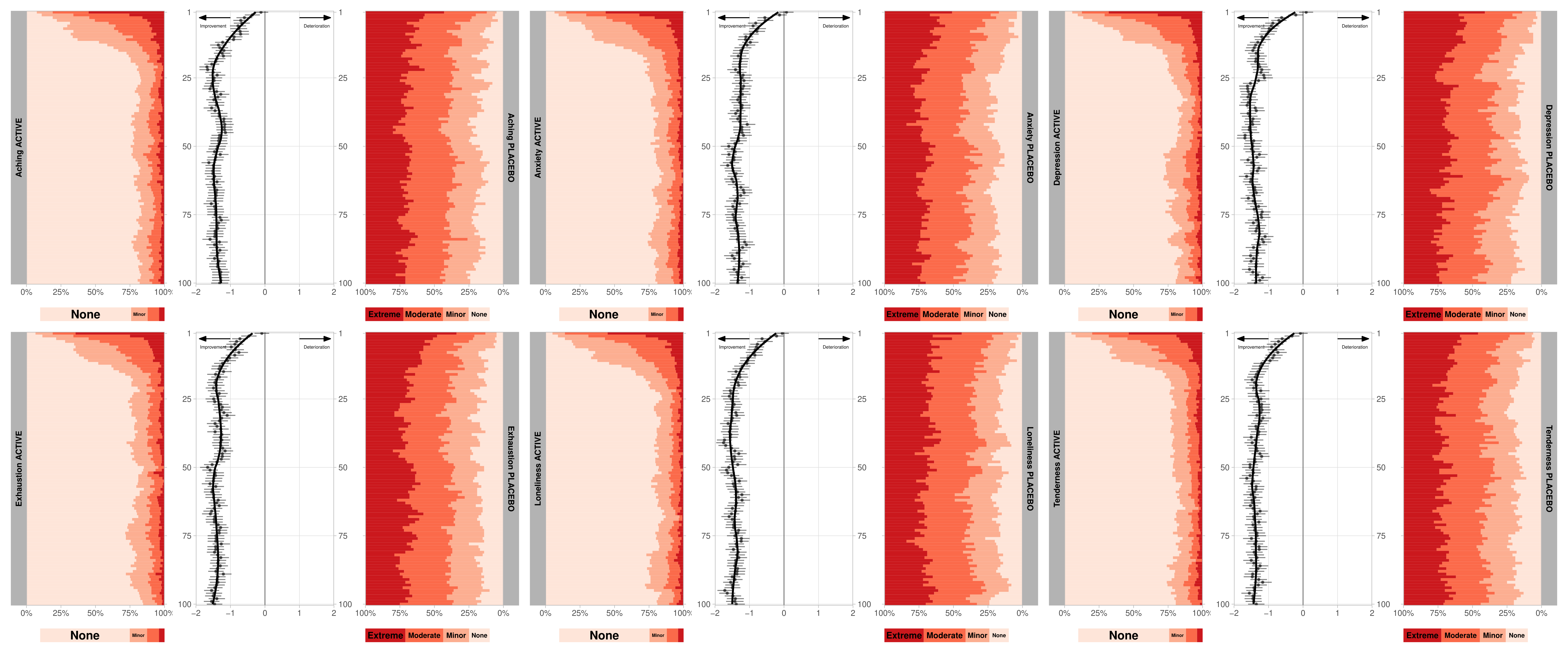
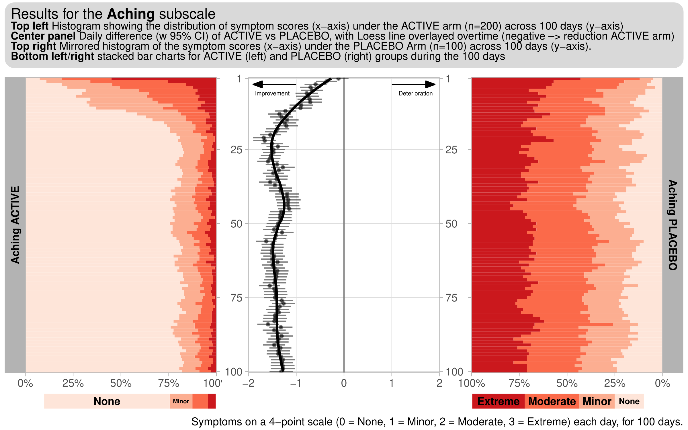
This month’s challenge will be to visualise diary data, whereby patients complete a diary (grading a number of symptoms), each day. For this challenge, we consider a hypothetical diary, consisting of 6 symptoms (Exhaustion, Aching, Tenderness, Depression, Loneliness, Anxiety). 300 subjects (200 active, 100 placebo), grade each of these symptoms on a 4-point scale (0 = None, 1 = Minor, 2 = Moderate, 3 = Extreme) each day, for 100 days.
Example 1.
(A summary of the discussion will be added shortly.)
Code
Example 1.
# packages
pacman::p_load(tidyverse, rio, labelled)
pacman::p_load(ggfittext)
pacman::p_load(ggh4x)
pacman::p_load(ggtext)

# working dir
setwd('C:/R/Wonderful-Wednesdays/2023-03-08')

# import
WWWDiary <- import("https://raw.githubusercontent.com/VIS-SIG/Wonderful-Wednesdays/master/data/2023/2023-03-08/WWWDiary.Rds")

# export
export(WWWDiary, 'WWWDiary.csv')
export(WWWDiary, 'WWWDiary.rds')

# transform
diary   <- WWWDiary %>%
   relocate(AVALC, .after = AVAL) %>%
   mutate(AVAL = as.numeric(AVAL)) %>%
   mutate(AVALC = factor(AVALC,
                         levels = c('None','Minor','Moderate','Extreme')) %>% fct_rev() )

# NEST T-TEST
diary_nest <- diary %>%
   nest_by(ADY, PARAM, PARAMN) %>%
   mutate(t.test = list( t.test(AVAL ~ TRT, data = data) %>%
                            broom::tidy() ) ) %>%
   select(-data) %>%
   unnest(cols = c(t.test))

# Differences
diary_d <- diary_nest %>%
   ungroup() %>%
   nest_by(PARAM, PARAMN) %>%
   mutate(gg_d = list(
      data %>%
         ggplot(aes(y = I(-1*ADY), x = estimate) ) +
         geom_vline(xintercept = 0, color = 'gray50') +
         geom_pointrange( aes(xmin = conf.low, xmax = conf.high),
                          size = 0.1,
                          alpha = .5) +
         geom_smooth(orientation = 'y', formula = y ~ x,
                     se = FALSE,  color = 'black', span = 0.35 ) +
         scale_y_continuous(name = NULL,
                            expand = c(0.005, 0.005),
                            labels = abs,
                            breaks = -1*c(1, 25, 50, 75, 100),
                            sec.axis = dup_axis() ) +
         scale_x_continuous(name = NULL,
                            limits = c(-2.0, 2.0),
                            expand = c(0, 0),
                            breaks = seq(-2, 2, 1) ) +

         annotate('segment',
                  arrow = arrow(angle = 20,
                                length = unit(0.05,"native"),
                                type = 'closed'),
                  x = -1, xend = -1.9,
                  y = -3, yend = -3) +

         annotate('segment',
                  arrow = arrow(angle = 20,
                                length = unit(0.05,"native"),
                                type = 'closed'),
                  x = 1, xend = 1.9,
                  y = -3, yend = -3) +

         annotate('text',
                  label = 'Improvement', size = 1.85,
                  x = -1.5,
                  y = -6) +

         annotate('text',
                  label = 'Deterioration', size = 1.85,
                  x = 1.5,
                  y = -6) +

         theme_light() +

         theme( panel.grid.minor = element_blank(),
                strip.background.y = element_blank(),
                strip.text.y = element_blank() )
      ) )

# Histogram (day)
diary_h <- diary %>%
   nest_by(PARAM, PARAMN, TRT) %>%
   mutate(data = list( data %>% mutate(PARAM = PARAM,
                                       TRT = TRT) ) ) %>%
   mutate(gg_h = list(
      ggplot(data = data,
             aes(y = I(-1*ADY), fill = AVALC)) +
         geom_histogram(binwidth  = 1, position = 'fill') +

         facet_wrap(str_glue("{PARAM} {str_to_upper(TRT)}") ~ .,
                    strip.position = ifelse(TRT == 'Active', "left", "right") ) +

         scale_x_continuous(name = NULL,
                            expand = c(0, 0),
                            labels = scales::percent,
                            trans = ifelse(TRT=='Active','identity','reverse')) +
         scale_y_continuous(name = NULL,
                            expand = c(0, 0),
                            labels = abs,
                            breaks = -1*c(1, 25, 50, 75, 100),
                            position = ifelse(TRT == 'Active', 'right', 'left') ) +
         scale_color_brewer(name = NULL,
                            palette = 'Reds',
                            direction = -1,
                            aesthetics = c("colour", "fill") ) +
         theme_light() +
         theme(panel.grid    = element_blank(),
               axis.text.y   = element_blank(),
               legend.position = "none",
               strip.text = element_text(color = "black",
                                         face = 'bold') ) )
   ) %>%
   mutate(gg_h2 = list(
      ggplot(data = data,
             aes(y = 1, fill = AVALC, label = AVALC) ) +

         geom_histogram(binwidth  = 1, position = 'fill') +

         geom_fit_text(stat="bin", binwidth  = 1, position="fill", fontface = 'bold', grow = TRUE) +

         scale_x_continuous(expand = c(0.04, 0.07),
                            trans = ifelse(TRT=='Active','identity','reverse')) +

         scale_y_continuous(expand = c(0, 0)) +

         scale_color_brewer(name = NULL,
                            palette = 'Reds',
                            direction = -1,
                            aesthetics = c("colour", "fill") ) +

         theme_void() +

         theme(legend.position = "none") ) )

# COMBINE
pacman::p_load(patchwork)

f1 <- (diary_h$gg_h[[1]] + diary_d$gg_d[[1]] + diary_h$gg_h[[2]]) /
   (diary_h$gg_h2[[1]] + plot_spacer() + diary_h$gg_h2[[2]]) + plot_layout(heights = c(20, 1) )

f2 <- (diary_h$gg_h[[3]] + diary_d$gg_d[[2]] + diary_h$gg_h[[4]]) /
   (diary_h$gg_h2[[3]] + plot_spacer() + diary_h$gg_h2[[4]])  + plot_layout(heights = c(20, 1) )

f3 <- (diary_h$gg_h[[5]] + diary_d$gg_d[[3]] + diary_h$gg_h[[6]]) /
   (diary_h$gg_h2[[5]] + plot_spacer() + diary_h$gg_h2[[6]])  + plot_layout(heights = c(20, 1) )

f4 <- (diary_h$gg_h[[7]] + diary_d$gg_d[[4]] + diary_h$gg_h[[8]]) /
   (diary_h$gg_h2[[7]] + plot_spacer() + diary_h$gg_h2[[8]])  + plot_layout(heights = c(20, 1) )

f5 <- (diary_h$gg_h[[9]] + diary_d$gg_d[[5]] + diary_h$gg_h[[10]]) /
   (diary_h$gg_h2[[9]] + plot_spacer() + diary_h$gg_h2[[10]])  + plot_layout(heights = c(20, 1) )

f6 <- (diary_h$gg_h[[11]] + diary_d$gg_d[[6]] + diary_h$gg_h[[12]]) /
   (diary_h$gg_h2[[11]] + plot_spacer() + diary_h$gg_h2[[12]])  + plot_layout(heights = c(20, 1) )

# EXPORT
ggsave(filename = 'WWWDiary.pdf',
       plot = (f1  | f2 | f3 ) / (f4 | f5 | f6) & theme( plot.margin = margin(6, 6, 6, 6, "pt") ),
       width = 24, height = 10)

# One subscale
f1 +
plot_annotation(
   title = '<span style = "font-size:12pt"> Results for the <b>Aching</b> subscale</span><br>
               **Top left** Histogram showing the distribution of symptom scores (x-axis) under the ACTIVE arm (n=200) across 100 days (y-axis)
               <br> **Center panel** Daily difference (w 95% CI) of ACTIVE vs PLACEBO, with Loess line overlayed overtime (negative --> reduction ACTIVE arm)
               <br> **Top right** Mirrored histogram of the symptom scores (x-axis) under the PLACEBO Arm (n=100) across 100 days (y-axis).
               <br> **Bottom left/right** stacked bar charts for ACTIVE (left) and PLACEBO (right) groups during the 100 days',
   caption  = 'Symptoms on a 4-point scale (0 = None, 1 = Minor, 2 = Moderate, 3 = Extreme) each day, for 100 days.') &
   theme( plot.margin = margin(2, 2, 2, 2, "pt"),
          plot.title = element_markdown(size = 9,
                                           fill = 'gray85',
                                           padding = margin(5, 5, 5, 5),
                                           r = grid::unit(8, "pt") ) )

ggsave(filename = 'WWWDiary_Aching.pdf',
       width = 8, height = 5)