Quality of life outcomes in a cancer trial: dealing with missing data
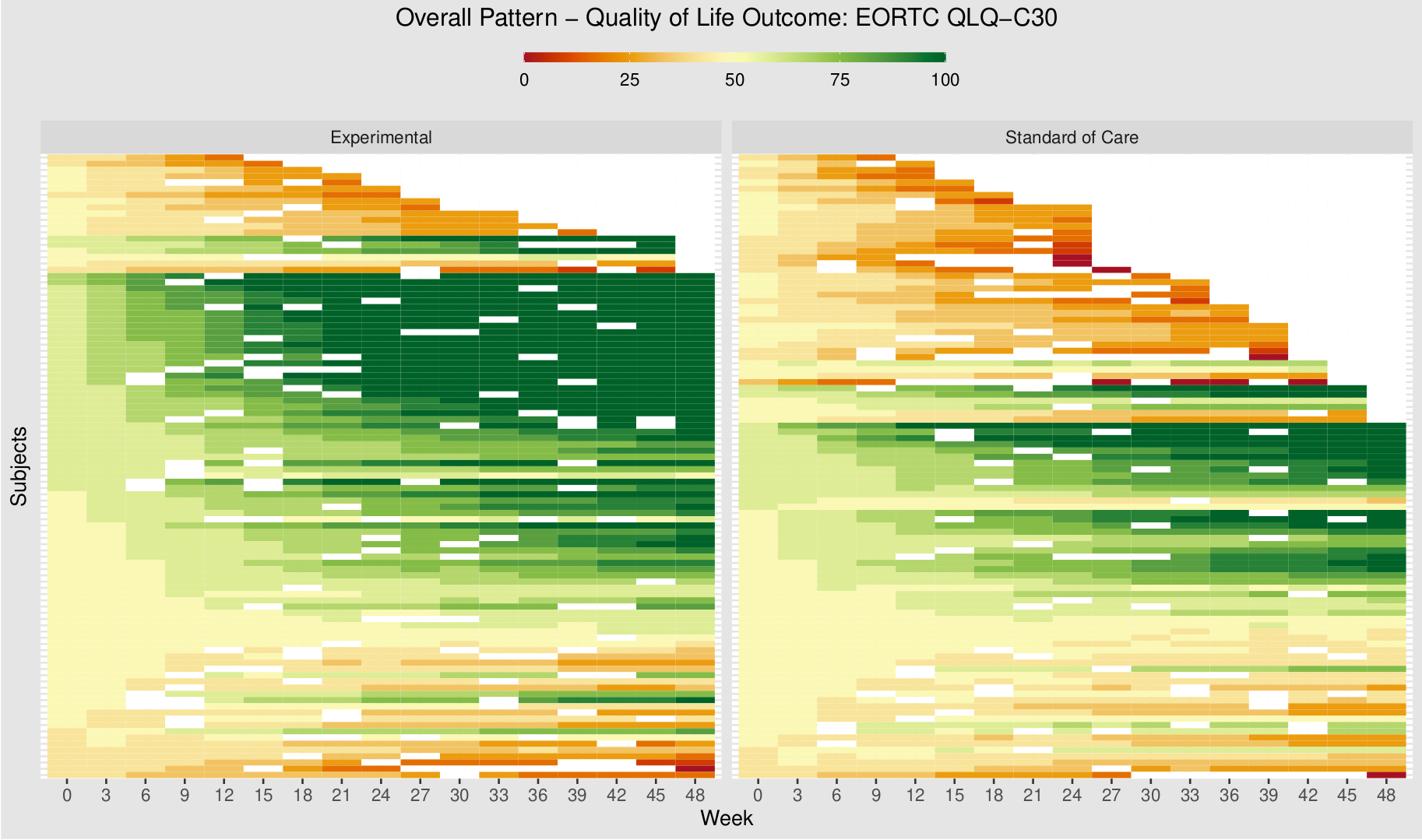
The EORTC QLQ-C30 is a 30-item questionnaire that has been designed for use in a wide range of cancer patient populations and is a reliable and valid measure of the quality of life in cancer patients. It includes a number of different scales, but this challenge is focussed on the global health and quality of life scale (QL).
A recording of the session can be found here.
Example 1.
Example 2.
Example 3.
Example 4.

Example 5.
Example 6.
high resolution image
high resolution image
high resolution image
high resolution image
high resolution image
Code
Example 1.
library(dplyr)
library(tidyr)
library(ggplot2)
library(forcats)
library(scales)
d0 <- read.csv2("ww eortc qlq-c30 missing.csv", sep=",") %>%
as_tibble()
d0
d1 <- df %>%
pivot_longer(cols=starts_with("WEEK"), names_to = "AVISIT", values_to = "AVAL") %>%
mutate(AVAL=as.numeric(AVAL)) %>%
select(USUBJID, ARM, LASTVIS, AGE:AVAL)
d1
d2 <- d1 %>%
group_by(ARM, LASTVIS, AVISIT) %>%
summarize(AVAL = mean(AVAL, na.rm=TRUE)) %>%
mutate(LASTVISC=as.factor(paste("Week", sprintf("%02.f", LASTVIS))),
AVISITN = as.numeric(gsub("WEEK","",AVISIT))) %>%
mutate(LASTVISC=fct_reorder(LASTVISC, LASTVIS))
cc <- scales::seq_gradient_pal("yellow", "blue", "Lab")(seq(0,1,length.out=14))
show_col(cc)
breaks <- sort(names(table(df_2$LASTVISC)))
labels <- breaks
ggplot(data=d2, aes(x=AVISITN, y=AVAL, group=LASTVISC, color=LASTVISC)) +
geom_line() +
geom_point() +
scale_y_continuous(breaks = round(seq(0, 100, 8.333333333),2),
limits = c(0, 100)) +
scale_x_continuous(breaks = seq(0, 48, 3), labels = paste("Wk", seq(0, 48, 3))) +
scale_color_manual(values = cc, labels=labels, breaks=breaks) +
facet_grid(cols=vars(ARM)) +
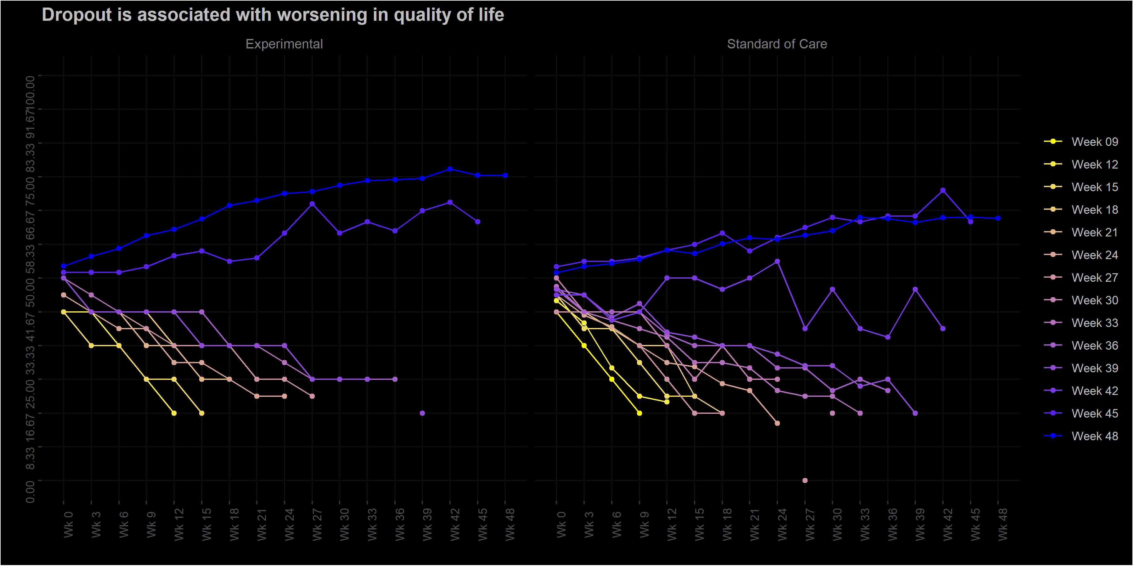
labs(title = "Dropout is associated with worsening in quality of life",
y = "EORTC QLQ-C30 QL [0-100]",
x = "Week on treatment") +
theme(plot.background = element_rect(fill="black"),
panel.background = element_rect(fill="black"),
legend.background = element_rect(fill="black"),
legend.box.background = element_rect(fill="black"),
legend.key = element_blank(),
legend.text = element_text(colour="grey"),
panel.grid = element_line(colour="grey5"),
panel.grid.minor = element_blank(),
strip.background = element_blank(),
plot.title=element_text(colour = "grey", size = 14, face = "bold"),
strip.text = element_text(colour = "grey50", size = 10),
axis.text = element_text(angle = 90))
ggsave(filename = "line_plot.png", device = "png", width = 12, height = 6)
Example 2.
No code has been submitted.
Example 3.
No code has been submitted.
Example 4.
library(dplyr)
library(tidyr)
library(ggplot2)
library(forcats)
library(scales)
library(ggalluvial)
library(RColorBrewer)

df <- read.csv2("ww eortc qlq-c30 missing.csv", sep=",") %>%
  as_tibble()
df
df_1 <- df %>%
  pivot_longer(cols=starts_with("WEEK"), names_to = "AVISIT", values_to = "AVAL") %>%
  select(USUBJID, ARM, LASTVIS, AGE:AVAL) %>%
  mutate(AVAL=as.factor(if_else(AVAL=="", "Missing", AVAL)))
df_1
levels(df_1$AVAL) <- c(as.character(rev(round(seq(0, 100, 8.333333333), 1))), "Missing")

cc <- scales::div_gradient_pal(low = "#a50026", mid="#ffffbf", high = "#313695", "Lab")(seq(0,1,length.out=13))

colors <- c(cc, "#D3D3D3")
show_col(colors)

ggplot(df_1,
       aes(
         x = AVISIT,
         stratum = AVAL,
         alluvium = USUBJID,
         fill = AVAL,
         label = AVAL
       )) +
  scale_fill_manual(values = colors) +
  scale_x_discrete(labels = paste("Wk", seq(0, 48, 3))) +

  geom_flow(stat = "alluvium",
            lode.guidance = "frontback",
            color = "darkgray") +
  geom_stratum() +
  labs(title = "Quality of Life - Missing data depends on age and treatment received") +
  facet_wrap(AGEGR~ARM, nrow = 4, scales = "free_y", strip.position = c("left")) +
  # facet_grid(cols = vars(ARM), rows = vars(AGEGR), scales = "free") +
  theme_bw() +
  guides(fill = guide_legend(nrow = 1, reverse = T)) +
  theme(
    #panel.background = element_blank(),
    #axis.text.y = element_blank(),
    legend.title = element_blank(),
    axis.title.x = element_blank(),
    legend.position = "bottom",
    strip.text = element_text(size = 12),
    axis.text = element_text(angle = 90),
    legend.direction = "horizontal"
  )

ggsave(filename = "sankey_chart.png", device = "png", width = 16, height = 9)
Example 5.
No code has been submitted.
Example 6.
No code has been submitted.