Sustained response data
Different approaches could be considered to define a patient as having sustained their response. A simple definition of sustained response could be that having achieved a response at a given visit, a patient then has that response at all subsequent visits. More complex approaches may explore different methods for interpolating between visits.
The dataset also contains a small amount of missing data. It may be of interest to explore how the approach used to handle this missing data influences the interpretation of sustained response.
Example 1. Lasagna plots
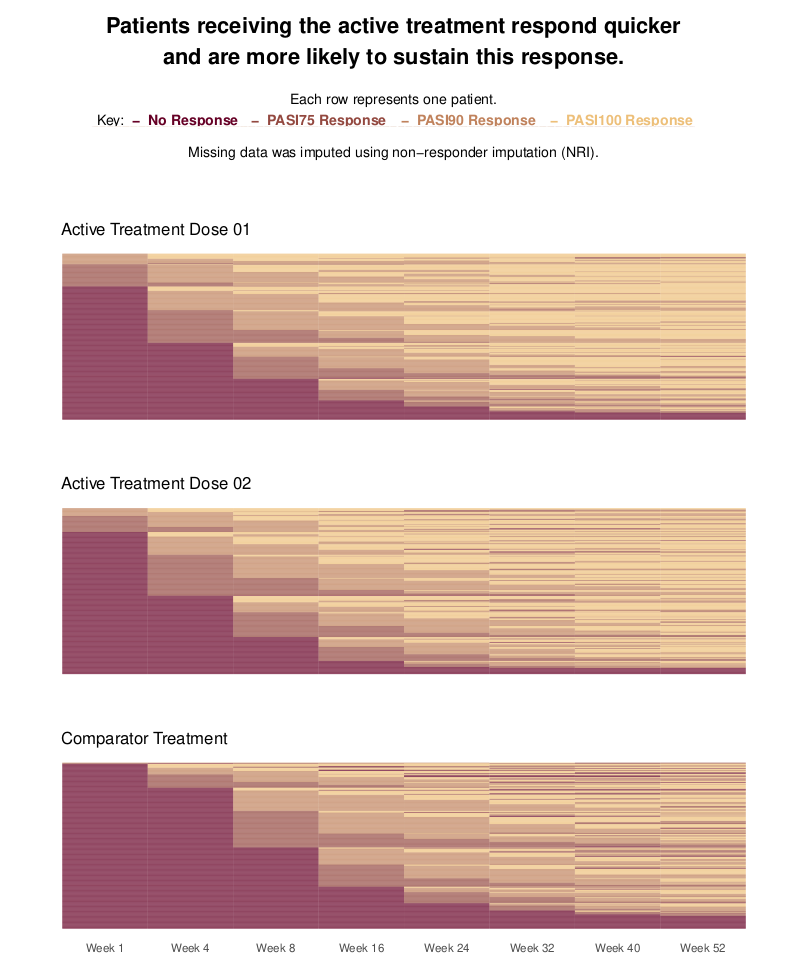
This visualization is based on patient level data and shows the PASI response over time. Each patient is represented by one line and the three groups are presented in three different blocks. The title is very clear and provides the reader with the main message. Furthermore, the color coding is presented (in the sub-title) as well as the imputation strategy. Therefore, it is very informative.
The selection of the colors is very reasonable. The colors go from red (no response) to yellow (PASI100) which makes intentionally sense considering that we are dealing with dermatology data. You can clearly see a step function over time and that the two active doses lead to a quicker response. Furthermore, at the right end of the plots, we see more yellow areas with the active doses than with the comparator.
The sorting of the patients is a challenge here. Even though the panelists considered the sorting as reasonable, there might be other options, for example, sorting by PASI100 at week 52. An interactive tool where the user can select the sorting might be an option and brings a lot of flexibility into this visualization.
Example 2. Dashboard with barplots
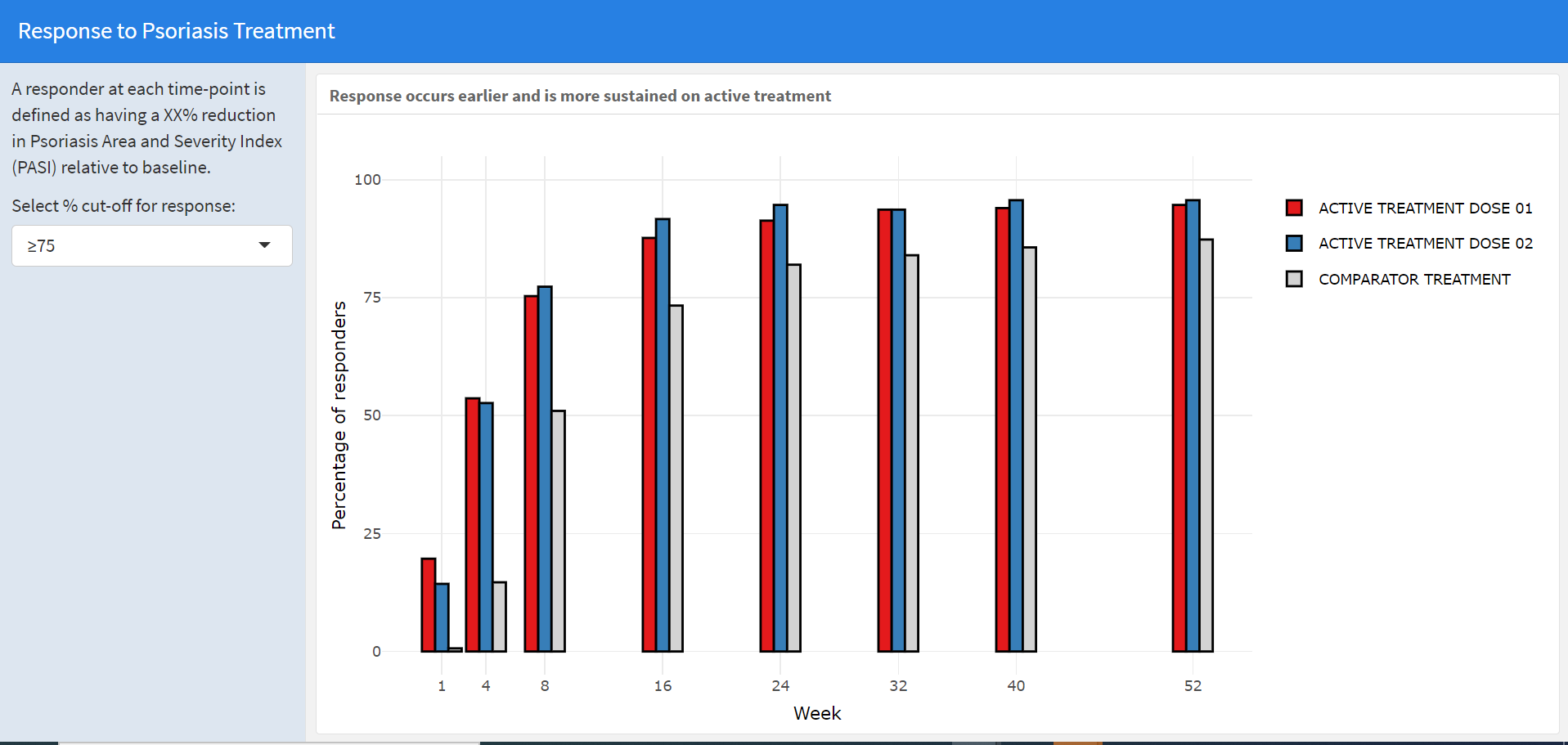
In the main panel, we see a barplot representing the percentage of responders over time. The groups are color-coded and can be easily distinguished due to the nice choice of colors. The (sub)title and the visualization itself have a clear message. Furthermore, the distance between the bars corresponds to the distance in time which is a nice detail.
This visualization has an interactive part: The user can select the percentage cut-off for response (in the left panel). When you select a different cut-off, the dimension of the y-axis remains the same which makes it very easy to compare the results even between the results based on different cut-offs. Furthermore, you can hover over the bars and it will provide you with additional information about the sustainability of the response.
(To use the app, just run the Rmd file in the “Code” section below.)
Example 3. Trajectory clustering
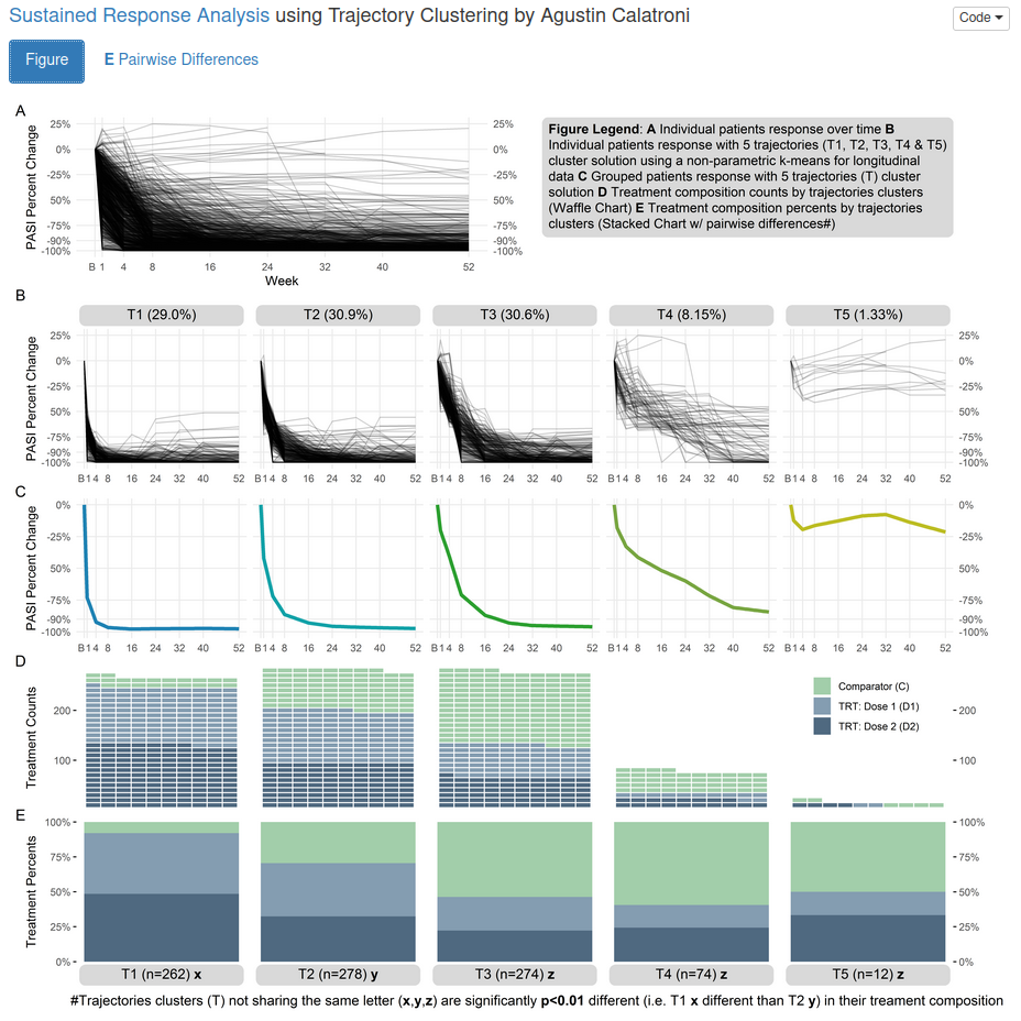
This is a very comprehensive visualization. Actually, it is not only a visualization, but also a presentation of a statistical analysis. A trajectory clustering has been performed to devide the patients into five different clusters with different characteristics in regards to their PASI percentage changes.
The row A presents the trajectories of all patients. This gives you a first overview over the data. In row B, the trajectories of the five clusters are provided. This gives you an overview over the different characteristics of the clusters. The first cluster seems to contain patients with a quick response and a very good sustainability of the response. This seems to be the cluster with the best performing patients. The second cluster is very similar, however, patients take a little longer until they respond and the overall level of the percentage change seems to be a bit worse. The third cluster is again a bit worse. The forth cluster still shows some improvement in PASI, however, quite many patients do not reach a good PASI response even at week 52. The fifth cluster contains patients who do not seem to improve in regards to the PASI score. (Note that there are only very few patients in this cluster.) Row C shows basically the same information as row B. An average trajectory per cluster is presented. Row D visualizes the number of patients per treatment group in each cluster using a “Waffle Chart”. And row E presents the percentages of patients per treatment group in each cluster.
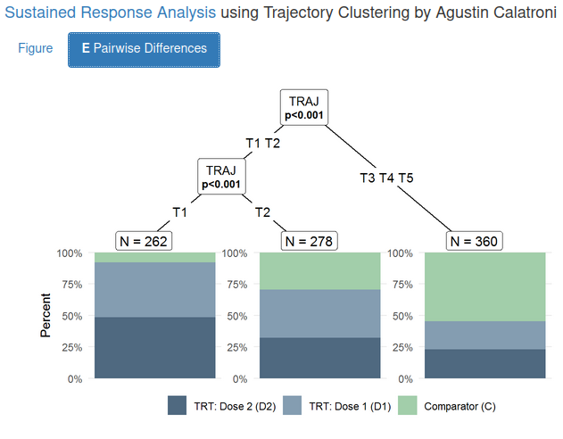
The boxes below the plots and the footnote provide additional information about the difference between cluster in their treatment composition. This information is further outlined in the second tab of the app. Using a tree, the differences in the treatment composition between the clusters is visualized.
This is a very interesting and useful analysis and visulization. You can see that the first cluster (which was the best one) contains mainly patients in the two active treatment arms. Thus, we can say that those treatments seem to lead to a quicker and a sustained response compared to the comparator. In the “worse” cluster, we see more patients who were in the comparator arm.
One aspect that could be improved is the coloring in row C. Actually, we do not need any color here, because the colors only seem to be different between the clusters. This information is already given by the structure of the columns, though. Furthermore, the colors are very similar to the colors which are used in row D and E to code the treatment arms.
Overall, this is a very elaborated and advanced visualization which provides the user with a lot of information. At the same time, the structure is very clear which makes it easy to understand the message of the visualization.
Code
Example 1. Lasagna plots
# Wonderful Wednesdays Submission - Sustained Response #

# Bring in data
SR_data <- read_excel("~/WWW/WWW_SustainedResponse_May.xlsx")

# Ensuring PASI score variables numeric
SR_data$BASELINE <- as.numeric(SR_data$BASELINE)
SR_data$WEEK01 <- as.numeric(SR_data$WEEK01)
SR_data$WEEK04 <- as.numeric(SR_data$WEEK04)
SR_data$WEEK08 <- as.numeric(SR_data$WEEK08)
SR_data$WEEK16 <- as.numeric(SR_data$WEEK16)
SR_data$WEEK24 <- as.numeric(SR_data$WEEK24)
SR_data$WEEK32 <- as.numeric(SR_data$WEEK32)
SR_data$WEEK40 <- as.numeric(SR_data$WEEK40)
SR_data$WEEK52 <- as.numeric(SR_data$WEEK52)

# Flags for different response levels

# Assigning value 3 for no response at any level
# A value of 2 for PASI75 response
# A value of 1 for PASI90 response
# A value of 0 for complete clearance
# Using NRI - Missing data assigned value 3
for(i in 1:length(SR_data$USUBJID)){

  if(is.na(SR_data$WEEK01[i])==TRUE){SR_data$WEEK01FL[i]=0}
  else if(SR_data$WEEK01[i]>0.25*SR_data$BASELINE[i]){SR_data$WEEK01FL[i]=0}
  else if(SR_data$WEEK01[i]>0.1*SR_data$BASELINE[i]){SR_data$WEEK01FL[i]=1}
  else if(SR_data$WEEK01[i]>0*SR_data$BASELINE[i]){SR_data$WEEK01FL[i]=2}
  else{SR_data$WEEK01FL[i]=3}

  if(is.na(SR_data$WEEK04[i])==TRUE){SR_data$WEEK04FL[i]=0}
  else if(SR_data$WEEK04[i]>0.25*SR_data$BASELINE[i]){SR_data$WEEK04FL[i]=0}
  else if(SR_data$WEEK04[i]>0.1*SR_data$BASELINE[i]){SR_data$WEEK04FL[i]=1}
  else if(SR_data$WEEK04[i]>0*SR_data$BASELINE[i]){SR_data$WEEK04FL[i]=2}
  else{SR_data$WEEK04FL[i]=3}

  if(is.na(SR_data$WEEK08[i])==TRUE){SR_data$WEEK08FL[i]=0}
  else if(SR_data$WEEK08[i]>0.25*SR_data$BASELINE[i]){SR_data$WEEK08FL[i]=0}
  else if(SR_data$WEEK08[i]>0.1*SR_data$BASELINE[i]){SR_data$WEEK08FL[i]=1}
  else if(SR_data$WEEK08[i]>0*SR_data$BASELINE[i]){SR_data$WEEK08FL[i]=2}
  else{SR_data$WEEK08FL[i]=3}

  if(is.na(SR_data$WEEK16[i])==TRUE){SR_data$WEEK16FL[i]=0}
  else if(SR_data$WEEK16[i]>0.25*SR_data$BASELINE[i]){SR_data$WEEK16FL[i]=0}
  else if(SR_data$WEEK16[i]>0.1*SR_data$BASELINE[i]){SR_data$WEEK16FL[i]=1}
  else if(SR_data$WEEK16[i]>0*SR_data$BASELINE[i]){SR_data$WEEK16FL[i]=2}
  else{SR_data$WEEK16FL[i]=3}

  if(is.na(SR_data$WEEK24[i])==TRUE){SR_data$WEEK24FL[i]=0}
  else if(SR_data$WEEK24[i]>0.25*SR_data$BASELINE[i]){SR_data$WEEK24FL[i]=0}
  else if(SR_data$WEEK24[i]>0.1*SR_data$BASELINE[i]){SR_data$WEEK24FL[i]=1}
  else if(SR_data$WEEK24[i]>0*SR_data$BASELINE[i]){SR_data$WEEK24FL[i]=2}
  else{SR_data$WEEK24FL[i]=3}

  if(is.na(SR_data$WEEK32[i])==TRUE){SR_data$WEEK32FL[i]=0}
  else if(SR_data$WEEK32[i]>0.25*SR_data$BASELINE[i]){SR_data$WEEK32FL[i]=0}
  else if(SR_data$WEEK32[i]>0.1*SR_data$BASELINE[i]){SR_data$WEEK32FL[i]=1}
  else if(SR_data$WEEK32[i]>0*SR_data$BASELINE[i]){SR_data$WEEK32FL[i]=2}
  else{SR_data$WEEK32FL[i]=3}

  if(is.na(SR_data$WEEK40[i])==TRUE){SR_data$WEEK40FL[i]=0}
  else if(SR_data$WEEK40[i]>0.25*SR_data$BASELINE[i]){SR_data$WEEK40FL[i]=0}
  else if(SR_data$WEEK40[i]>0.1*SR_data$BASELINE[i]){SR_data$WEEK40FL[i]=1}
  else if(SR_data$WEEK40[i]>0*SR_data$BASELINE[i]){SR_data$WEEK40FL[i]=2}
  else{SR_data$WEEK40FL[i]=3}

  if(is.na(SR_data$WEEK52[i])==TRUE){SR_data$WEEK52FL[i]=0}
  else if(SR_data$WEEK52[i]>0.25*SR_data$BASELINE[i]){SR_data$WEEK52FL[i]=0}
  else if(SR_data$WEEK52[i]>0.1*SR_data$BASELINE[i]){SR_data$WEEK52FL[i]=1}
  else if(SR_data$WEEK52[i]>0*SR_data$BASELINE[i]){SR_data$WEEK52FL[i]=2}
  else{SR_data$WEEK52FL[i]=3}

}

# Dataset for each treatment arm and sorting by response level at each visit

# Active Treatment Arm Dose 01

actarm01 <- SR_data %>% filter(TRT=='ACTIVE TREATMENT DOSE 01')
actarm01 <- actarm01[order(actarm01$WEEK01FL, actarm01$WEEK04FL, actarm01$WEEK08FL,
                           actarm01$WEEK16FL, actarm01$WEEK24FL, actarm01$WEEK32FL,
                           actarm01$WEEK40FL, actarm01$WEEK52FL),]
actarm01$subjord <- seq(from=1, to=300)
actarm01 <- actarm01 %>% dplyr::select(USUBJID, subjord, WEEK01FL, WEEK04FL, WEEK08FL, WEEK16FL,
                                WEEK24FL, WEEK32FL, WEEK40FL, WEEK52FL)

# Convert to long format
actarm01 <- gather(actarm01, visit, colour, WEEK01FL:WEEK52FL)
actarm01 <- actarm01[order(actarm01$subjord),]
# Evenly spaced bars for each visit
actarm01$bheight <- 1

act1plot <- ggplot() + scale_y_continuous(limits = c(0, 8), breaks = c(0.5,7.5),
                                          labels = c("0.5"="", "7.5" = "")) +
  geom_bar(data = actarm01, mapping = aes(x = subjord, y = bheight, fill = colour), stat = "identity", position = position_stack(reverse = TRUE), show.legend = TRUE) +
  coord_flip() + theme_bw() + theme_bw() + theme(panel.border = element_blank(), panel.grid.major = element_blank(),
                                                                                                                          panel.grid.minor = element_blank()) +
  theme(axis.ticks.x = element_blank(),
        axis.ticks.y = element_blank(),
        axis.text.y = element_blank()) + labs(x = "", y = "") +
  scale_fill_continuous(low="#660025", high="#edbf79", guide=FALSE) + labs(title="       Active Treatment Dose 01")


# Active Treatment Dose 02

actarm02 <- SR_data %>% filter(TRT=='ACTIVE TREATMENT DOSE 02')
actarm02 <- actarm02[order(actarm02$WEEK01FL, actarm02$WEEK04FL, actarm02$WEEK08FL,
                           actarm02$WEEK16FL, actarm02$WEEK24FL, actarm02$WEEK32FL,
                           actarm02$WEEK40FL, actarm02$WEEK52FL),]
actarm02$subjord <- seq(from=1, to=300)
actarm02 <- actarm02 %>% dplyr::select(USUBJID, subjord, WEEK01FL, WEEK04FL, WEEK08FL, WEEK16FL,
                                       WEEK24FL, WEEK32FL, WEEK40FL, WEEK52FL)

actarm02 <- gather(actarm02, visit, colour, WEEK01FL:WEEK52FL)
actarm02 <- actarm02[order(actarm02$subjord),]
actarm02$bheight <- 1


act2plot <- ggplot()  + scale_y_continuous(limits = c(0, 8), breaks = c(0.5, 7.5),
                                           labels = c("0.5"="", "7.5" = "")) +
  geom_bar(data = actarm02, mapping = aes(x = subjord, y = bheight, fill = colour), stat = "identity", position = position_stack(reverse = TRUE), show.legend = TRUE) +
  coord_flip() + theme_bw() + theme_bw() + theme(panel.border = element_blank(), panel.grid.major = element_blank(),
                                                 panel.grid.minor = element_blank()) +
  theme(axis.ticks.x = element_blank(),
        axis.ticks.y = element_blank(),
        axis.text.y = element_blank()) + labs(x = "", y = "") +
  scale_fill_continuous(low="#660025", high="#edbf79", guide=FALSE)+ labs(title="       Active Treatment Dose 02")

# Comparator Treatment
comparm <- SR_data %>% filter(TRT=='COMPARATOR TREATMENT')
comparm <- comparm[order(comparm$WEEK01FL, comparm$WEEK04FL, comparm$WEEK08FL,
                         comparm$WEEK16FL, comparm$WEEK24FL, comparm$WEEK32FL,
                         comparm$WEEK40FL, comparm$WEEK52FL),]
comparm$subjord <- seq(from=1, to=300)
comparm <- comparm %>% dplyr::select(USUBJID, subjord, WEEK01FL, WEEK04FL, WEEK08FL, WEEK16FL,
                                     WEEK24FL, WEEK32FL, WEEK40FL, WEEK52FL)

comparm <- gather(comparm, visit, colour, WEEK01FL:WEEK52FL)
comparm <- comparm[order(comparm$subjord),]
comparm$bheight <- 1


compplot <- ggplot()  + scale_y_continuous(limits = c(0, 8), breaks = c(0.5,1.5,2.5,3.5,4.5,5.5,6.5,7.5),
                                           labels = c("0.5"="Week 1", "1.5" = "Week 4", "2.5" = "Week 8", "3.5" = "Week 16",
                                                      "4.5" = "Week 24", "5.5" = "Week 32", "Week 6.5" = "Week 40", "7.5" = "Week 52")) +
  geom_bar(data = comparm, mapping = aes(x = subjord, y = bheight, fill = colour), stat = "identity", position = position_stack(reverse = TRUE), show.legend = TRUE) +
  coord_flip() + theme_bw() + theme_bw() + theme(panel.border = element_blank(), panel.grid.major = element_blank(),
                                                 panel.grid.minor = element_blank()) +
  theme(axis.ticks.x = element_blank(),
        axis.ticks.y = element_blank(),
        axis.text.y = element_blank()) + labs(x = "", y = "") +
  scale_fill_continuous(low="#660025", high="#edbf79", guide=FALSE)+ labs(title="       Comparator Treatment")

# Plotting together

text1 = paste("Patients receiving the active treatment respond quicker\nand are more likely to sustain this response.\n\n\n")
text2 = paste("\nEach row represents one patient.")
text3 = paste("\n\n\nKey:________________________________________________________________________")
text4 = paste("\n\n\n_____-_No Response__________________________________________________________")
text5 = paste("\n\n\n____________________-_PASI75 Response_______________________________________")
text6 = paste("\n\n\n_______________________________________-_PASI90 Response____________________")
text7 = paste("\n\n\n__________________________________________________________-_PASI100 Response")
# White overlay to cover coloured underscores used for spacing
text8 = paste("\n\n\n___________________________________________________________________________________")
text9 = paste("\n\n\n\n\n\nMissing data was imputed using non-responder imputation (NRI).")
blankplot <- ggplot() +
  annotate("text", x = 4, y = 25, size=6, label = text1, fontface='bold') +
  annotate("text", x = 4, y = 25, size=4, label = text2) +
  annotate("text", x = 4, y = 25, size=4, label = text3) +
  annotate("text", x = 4, y = 25, size=4, label = text4, col="#660025", fontface='bold') +
  annotate("text", x = 4, y = 25, size=4, label = text5, col="#93483f", fontface='bold') +
  annotate("text", x = 4, y = 25, size=4, label = text6, col="#c0825c", fontface='bold') +
  annotate("text", x = 4, y = 25, size=4, label = text7, col="#edbf79", fontface='bold')+
  annotate("text", x = 4, y = 25, size=4, label = text8, col="white", fontface='bold') +
  annotate("text", x = 4, y = 25, size=4, label = text8, col="white", fontface='bold') +
  annotate("text", x = 4, y = 25, size=4, label = text8, col="white", fontface='bold') +
  annotate("text", x = 4, y = 25, size=4, label = text8, col="white", fontface='bold') +
  annotate("text", x = 4, y = 25, size=4, label = text8, col="white", fontface='bold') +
  annotate("text", x = 4, y = 25, size=4, label = text9) +
  theme_void()


# Multiplot function taken from cookbook for r:
# http://www.cookbook-r.com/Graphs/Multiple_graphs_on_one_page_%28ggplot2%29/

multiplot <- function(..., plotlist=NULL, file, cols=1, layout=NULL) {
  library(grid)

  # Make a list from the ... arguments and plotlist
  plots <- c(list(...), plotlist)

  numPlots = length(plots)

  # If layout is NULL, then use 'cols' to determine layout
  if (is.null(layout)) {
    # Make the panel
    # ncol: Number of columns of plots
    # nrow: Number of rows needed, calculated from # of cols
    layout <- matrix(seq(1, cols * ceiling(numPlots/cols)),
                     ncol = cols, nrow = ceiling(numPlots/cols))
  }

  if (numPlots==1) {
    print(plots[[1]])

  } else {
    # Set up the page
    grid.newpage()
    pushViewport(viewport(layout = grid.layout(nrow(layout), ncol(layout))))

    # Make each plot, in the correct location
    for (i in 1:numPlots) {
      # Get the i,j matrix positions of the regions that contain this subplot
      matchidx <- as.data.frame(which(layout == i, arr.ind = TRUE))

      print(plots[[i]], vp = viewport(layout.pos.row = matchidx$row,
                                      layout.pos.col = matchidx$col))
    }
  }
}

#Final Plot
multiplot(blankplot, act1plot, act2plot, compplot)
Example 2. Dashboard with barplots
Example 3. Trajectory clustering