Progression free survival

Background

The example simulated data set is based on large phase III clinical trials in Breast cancer such as ALTTO.

The “trial” aims to determine if a combination of two therapies tablemab (T) plus vismab (V) improves outcomes for metastatic human epidermal growth factor 2–positive breast cancer and increases the pathologic complete response in the neoadjuvant setting (treatment given as a first step to shrink a tumor before the main treatment or surgery).

The trial has four treatment arms, patients with centrally confirmed human epidermal growth factor 2-positive early breast cancer were randomly assigned to 1 year of adjuvant therapy with V, T, their sequence (T→V), or their combination (T+V) for 52 weeks. The primary end point was progression-free survival (PFS).

As defined by Cancer.gov: “the length of time during and after the treatment of a disease, such as cancer, that a patient lives with the disease but it does not get worse. In a clinical trial, measuring the progression-free survival is one way to see how well a new treatment works”.

The data set and variable definitions

The data set is an abridged version of the CDISC ADaM ADTTE time to event data set.

The data set contains the following variables:

• STUDYID - the study identifier
• SUBJID - subject identifier
• USUBJID - unique subject iddentifier
• AGE - age at randomisation (years)
• STR01 - Hormone receptor status at randomisation
• STR01N - Hormone receptor positive (Numeric)
• STR01L - Hormone receptor positive (Long format)
• STR02 - Prior Radiotherapy at randomisation
• STR02N - Prior Radiotherapy at randomisation (Numeric)
• STR02L - Prior Radiotherapy at randomisation (Long format)
• TRT01P - Planned treatment assigned at randomisation
• TRT01PN - Planned treatment assigned at randomisation (Numeric)
• PARAM - Analysis parameter - Progression free survival
• PARAMCD - Analysis parameter code
• AVAL - Analysis value (time to event [days])
• CNSR - Censoring (0 = Event, 1 = censored)
• EVNTDESC - Event description
• CNSDTDSC - Censoring description
• DCTREAS - Discontinuation from study reason

A number of baseline measurements are also included such as age, hormone receptor status and prior radiotherapy treatment. Additional details on reasons for study discontinuation and censoring event description are also included.

Challenge

Visualise the pattern of events (disease progression, death, etc) on a summary data level or on a patient level data. Highlight differences between treatments or subgroups.

Example analysis

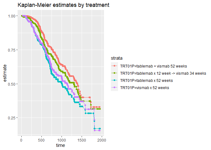
Below is a crude example of how to work with the CDISC ADaM ADTTE data set. The example takes the AVAL, CNSR and TRT01P variables to plot Kaplan-Meier estimates by treatment.

library(tidyverse)    
library(broom)
library(survival)

# load data
ADTTE <- read_csv('2024-08-12-psi-vissig-adtte.csv')

# plot KM curve by treatment 
survfit(Surv(AVAL, CNSR == 0) ~ TRT01P  , data = ADTTE )  %>%
  tidy(fit) %>%
  ggplot(aes(time, estimate, group = strata, colour = strata)) + 
  geom_line() +
  geom_point() +
  ggtitle("Kaplan-Meier estimates by treatment")