Wonderful-Wednesdays
Repository to hold the data and materials for the Wonderful Wednesday webinar series https://www.psiweb.org/sigs-special-interest-groups/visualisation/welcome-to-wonderful-wednesdays
Example meta-analysis dataset
Purpose
The purpose of this webinar is to explore how data visualisation can be deployed to find insights when faced with big data.
For this webinar, we introduce the challenge of working with pooled or integrated clinical trial data. This is often referred to as meta-analysis.
Key issues where data visualisation can help are around the investigation of whether studies can be combined due to study heterogeneity among individual trials. This throws up questions such as:
- What graphical tools can be used to assess heterogeneity, describing the fixed and random-effects?
- what variables are potentially prognostic or predictive of outcome, etc?
- where can graphical methods provide some general recommendations?
Background
Meta-analysis are a popular approach for summarising a large number of clinical trials. We can resolving discrepancies raised by individual these trials, identify new insights, or attempt to tackle new research questions.
The example simulated data set for this challenge is based on seven phase III studies in Hypertension. The objective of the studies were to compare the use of intensive hypertensive medicines to control blood pressure compared to standard of care. The studies are inspired by the large blood pressure intervention studies such as SPRINT.
In this case, instead of a large single trial, we are faced with an integreted set of seven seperate trials.
The integrated data
The data set is an abridged version of CDISC ADaM.
The data set contains the following key variables for analysis:
- STUDYID Masked study identifer
- USUBJD Masked subject identifier Identifer
- TRT01P Randomised treatment
- AVAL Mean systolic blood pressure (mm Hg) measured at 1-year
- BASE Mean systolic blood pressure (mm Hg) measured at baseline
- CHG Change from baseline mean systolic blood pressure (SBP) [mm Hg] at 1-year
- PCHG Percentage change from baseline mean systolic blood pressure (%change) at 1-year
- AVALCAT1 Responder analysis - patients with controlled SBP at 1-Year (<=120 mmHg) 1 = Yes, 0 = No 1-Year
A wide collection of baseline measurements are also included which can be explored to understand the patient populations within each trial, to search for potential subgroups or differential treatment effects, or even to develop prognostic or predictive risk models.
For a detailed overview of the data set, please refer to the data dictionary section below (or in the file that can be downloaded here).
Outcome - contolled blood pressure at 1-year
The outcome variable AVAL is the mean systolic blood pressure (mm Hg) measured at 1-year. This is an average of three in clinic measurements. A corresponding measurement taken at baseline BASE is also provided that could be used as a covariate.
Additional potential outcome variables are provided such as the change score CHG and percentage change score PCHG between baseline and 1-year.
Other outcomes based around the key outcome measure include a typical responder analysis to determine how many patients are below the criteria of Hyptertension (120 mmHG) at 1-year.
Data Dictionary
In this section is a description of all variables.
| Variable name | Description | Assessment Visit |
|---|---|---|
| STUDYID | Masked study identifer | Identifer |
| USUBJD | Masked subject identifier | Identifer |
| TRT01P | Randomised treatment | Treatment |
| TRT01PC | Randomised treatment (Character) | Treatment |
| TRT01PN | Randomised treatment (Numeric) | Treatment |
| PARAM | Analysis variable label | 1-Year |
| AVAL | Mean systolic blood pressure (mm Hg) measured at 1-Year | 1-Year |
| CHG | Change from baseline Mean systolic blood pressure (mm Hg) | 1-Year |
| PCHG | Percentage change from baseline Mean systolic blood pressure (%change) | 1-Year |
| AVALCAT1 | Responder analysis - patients with controlled SBP at 1-Year (<=120 mmHg) 1 = Yes, 0 = No | 1-Year |
| AVALCAT1N | Responder analysis - patients with controlled SBP at 1-Year (<=120 mmHg) 1 = Yes, 0 = No | 1-Year |
| AVALCAT2 | Mean systolic blood pressure (mm Hg) measured at 1-Year categories (<= 132, 132 - 145, >= 145) | 1-Year |
| AVALCAT2N | Mean systolic blood pressure (mm Hg) measured at 1-Year categories (numeric) (<= 132, 132 - 145, >= 145) | 1-Year |
| AGE | Age (years) | Baseline |
| AGECAT1 | Age Group 3: 75 years and older = TRUE | Baseline |
| AGECAT1C | Age Group 3: 75 years and older = TRUE | Baseline |
| AGECAT1N | Age Group 3: 75 years and older = TRUE | Baseline |
| ALBSI | Albumin (g/L) | Baseline |
| BASE | Mean systolic blood pressure (mm Hg) measured at baseline | Baseline |
| BASOSI | Basophils (Absolute) (10E9/L) | Baseline |
| BICARSI | Bicarbonate (mmol/L) | Baseline |
| BILISI | Bilirubin (umol/L) | Baseline |
| BMI | BMI | Baseline |
| BUNSI | Blood Urea Nitrogen (mmol/L) | Baseline |
| CASI | Calcium (mmol/L) | Baseline |
| CHD10R1 | 10-year Coronary heart disease (CHD) risk category (High (>20%) , Medium (10-20%), Low (<10%)) | Baseline |
| CHD10R1N | 10-year CHD risk category (Numeric, 1 = Low, 2 = Medium, 3 = High) | Baseline |
| CHOL_HDL | Ratio of Total Cholesterol / HDL | Baseline |
| CHOLSI | Cholesterol (mmol/L) | Baseline |
| COUNTRY | Country indicator | Baseline |
| CREATSI | Creatinine (umol/L) | Baseline |
| EOSLESI | Eosinophils/Leukocytes (%) | Baseline |
| EOSSI | Eosinophils (Absolute) (10E9/L) | Baseline |
| ETHNIC | Ethnicity | Baseline |
| GGTSI | Gamma Glutamyl Transferase (U/L) | Baseline |
| GLUCPSI | Glucose, Plasma, Fasting (mmol/L) | Baseline |
| GREGGR1O | Regional stratification group | Baseline |
| HCT | Hematocrit | Baseline |
| HDLSI | HDL Cholesterol (mmol/L) | Baseline |
| HDT | Phosphate (mmol/L) | Baseline |
| HEIGHT | Height (cm) | Baseline |
| HGBSI | Hemoglobin (g/L) | Baseline |
| KSI | Potassium (mmol/L) | Baseline |
| LDLSI | LDL Cholesterol (Assayed) (mmol/L) | Baseline |
| LPASI | Lipoprotein-A Protein (g/L) | Baseline |
| LYMLESI | Lymphocytes/Leukocytes (%) | Baseline |
| LYMSI | Lymphocytes (Absolute) (10E9/L) | Baseline |
| MONOLSI | Monocytes/Leukocytes (%) | Baseline |
| RACE | Race | Baseline |
| SBPCAT1C | Mean systolic blood pressure (mm Hg) at baseline (Category) | Baseline |
| SBPCAT1N | Mean systolic blood pressure (mm Hg) at baseline (Numeric) | Baseline |
| SEX | Sex | Baseline |
| TRIGFSI | Triglycerides (Fasting) (mmol/L) | Baseline |
| URATESI | Uric Acid (umol/L) | Baseline |
| WBCSI | Leukocytes (10E9/L) | Baseline |
| WEIGHT | Weight (kg) | Baseline |
Downloading data
NOTE to download a single data set as a csv file, click on the raw button and save the file. The following link describes the process in further detail.
Example analysis
This section illustrates a simple example analysis.
Load data
library(tidyverse)
library(broom)
data <- read_csv("BIG_DATA_PSI_WW_DEC2020.csv")
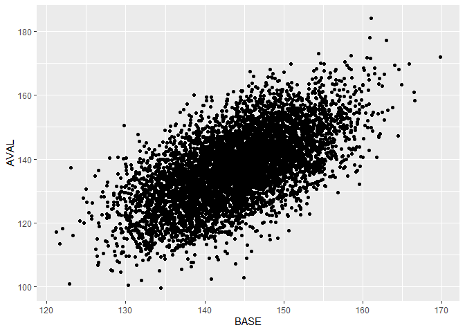
Plot pooled data
Plot the pre-post mean systolic blood pressure of all patients for all studies.
data %>% ggplot(aes(x = BASE, y = AVAL)) +
  geom_point()
Simple analysis by study
A between study comparison of intensive treatment vs standard of care.
data %>%
  group_by(STUDYID) %>%
  do(fit = tidy(lm(AVAL ~ BASE + TRT01PN, data = .))) %>%
  unnest(fit) %>%
  filter(term == "TRT01PN")
## # A tibble: 7 x 6
##   STUDYID term    estimate std.error statistic  p.value
##     <dbl> <chr>      <dbl>     <dbl>     <dbl>    <dbl>
## 1       1 TRT01PN    -7.12     0.480     -14.8 5.14e-44
## 2       2 TRT01PN    -8.17     0.694     -11.8 1.60e-28
## 3       3 TRT01PN   -10.1      0.508     -19.8 5.97e-73
## 4       4 TRT01PN    -7.27     0.476     -15.3 3.18e-48
## 5       5 TRT01PN    -6.97     0.665     -10.5 1.57e-23
## 6       6 TRT01PN    -6.80     0.358     -19.0 4.40e-74
## 7       7 TRT01PN    -7.74     0.621     -12.5 2.48e-32
Across all studies, there is evidence to suggest intensive treatment improves blood pressure control (decreases blood pressure) at 1-year compared to standard of care.